Evidence Sensitivity Analysis

What is Evidence Sensitivity Analysis?

Evidence sensitivity analysis (SE analysis) is the analysis of how sensitive the results of a belief update (propagation of evidence) is to variations in the set of evidence (observations, likelihood, etc.).

Consider the situation where a decision maker has to make a decision based on the probability distribution of a hypothesis variable. It could, for instance, be a physician deciding on a treatment of a patient given the probability distribution of a disease variable. Prior to deciding on a treatment the physician may have the option to investigate the impact of the collected information on the posterior distribution of the hypothesis variable. Given a set of findings and a hypothesis, which sets of findings are in favor, against, or irrelevant for the hypothesis, which sets of findings discriminate the hypothesis from an alternative hypothesis, what if a variable had been observed to a different value than the one observed, etc. These questions can be answered by SE analysis.

Given a Bayesian network model and a hypothesis variable, the task is to determine how sensitive the belief in the hypothesis variable is to variations in the evidence. We consider myopic hypothesis driven SE analysis on discrete random variables.

Evidence sensitivity analysis is available for discrete chance nodes only if there are no unpropagated evidence. The functionality is enabled when a discrete chance node is selected or when pressing the right mouse button on a discrete chance node in the Node List Pane.

Distance Measures

The main purpose of hypothesis driven SE analysis is to investigate how changes in the set of evidence impact the probability of a hypothesis. In order to perform this investigation two distance measures are required. Each distance measure will provide a numerical value specifying the distance between either two probabilities or two probability distributions.

Let X be a hypothesis variable with state space x₁,…,x_n and let \(\varepsilon\) = { \(\varepsilon_1\), …, \(\varepsilon_m\)} be a set of evidence (findings). We let \(\varepsilon_Y\) in \(\varepsilon\) denote the finding on variable Y in X(\(\varepsilon\)).

The distance d(p,q) between two probabilities p and q is defined, for p different from zero, as:

\[d(p, q) = |\frac{q}{p} - 1|\]

This measure is, for instance, useful for measuring the distance between the probability P(x| \(\varepsilon\)) of hypothesis x given evidence \(\varepsilon\) and the probability P(x| \(\varepsilon\){ \(\varepsilon_i\)}) of hypothesis x given evidence \(\varepsilon\){ \(\varepsilon_i\)}, i.e., the set of evidence where \(\varepsilon_i\) is excluded from \(\varepsilon\).

A pair of probabilities p and q are said to be almost equal when their distance d(p,q) is below a predefined threshold \(\delta\), i.e., d(p,q) < \(\delta\).

The cost-of-omission c(P(X| \(\varepsilon\)), P(X| \(\varepsilon\){ \(\varepsilon_i\)})) of \(\varepsilon_i\) is defined as:

\[c(P| X| \varepsilon), P(X| \varepsilon \setminus \{ \varepsilon_i\}) = \sum_{x \in dom(x)} P(X | \varepsilon) log(\frac{P(x| \varepsilon)}{P(x| \varepsilon \setminus \{\varepsilon_i\})})\]

This formula is undefined for values P(x| \(\varepsilon\))=0 and P(x| \(\varepsilon\){ \(\varepsilon_i\)})=0. For these two cases, we define cost-of-omission to be 0 and infinity, respectively. Notice the difference between the distance measure and the cost-of-omission measure. The distance measure evaluates the distance between probability values whereas the cost-of-omission measure evaluates the distance between two posterior probability distributions relative to omitting a certain finding \(\varepsilon_i\) from the evidence \(\varepsilon\). The cost-of-omission measure is a special case of the more general cross entropy distance (or Kullback-Leibler distance) measure between a probability distribution P and an approximation P’ of P:

\[H(P, P') = \sum_{x \in dom(x)} P(x) log(\frac{P(x)}{P'(x)})\]

The cost-of-omission measure is, for instance, useful for measuring the distance between the posterior probability distribution P(X| \(\varepsilon\)) of hypothesis variable X given evidence \(\varepsilon\) and the posterior probability distribution P(X| \(\varepsilon\){\(\varepsilon_i\)}) of hypothesis variable X given evidence \(\varepsilon\){\(\varepsilon_i\)}, i.e., the set of evidence where \(\varepsilon_i\) is excluded from \(\varepsilon\).

Min-Max

As part of performing a SE analysis we may be interested in knowing the minimum and maximum values of the posterior belief in each possible state of the hypothesis variable given all possible observations on a given variable.

Using the dialog shown in Figure 1 we may for each information variable determine the minimum, current, and maximum value of the posterior probability of each state of the hypothesis variable. The minimum and maximum values are determined by entering and propagating each state of the information variable. This analysis requires one propagation for each state of each possible information variable.

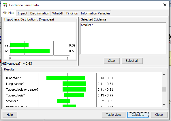
Figure 1: The entropy of the hypothesis variable B is H(B)=0.63.

Figure 1 shows the posterior probability distribution of Has bronchitis given the entire set of evidence, the entropy H(Has bronchitis)=0.63 of Dyspnoea? as well as the minimum, current, and maximum values for the posterior probability of Dyspnoea equal to yes given variations over each selected information variable (i.e., Has bronchitis, Tuberculosis or cancer, etc).

Pressing the Table View button in the dialog shown in Figure 1 produces the table shown in Figure 2.

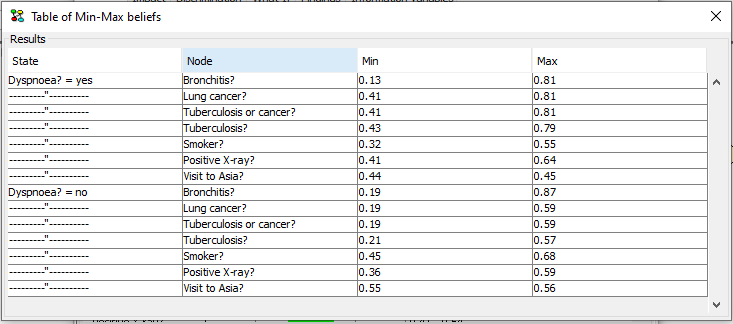
Figure 2: Table view of the results in Figure 1.

Impact

Investigation of the impact of different subsets of the evidence on each state of the hypothesis variable is a useful part of SE analysis. Investigating the impact of different subsets of the evidence on states of the hypothesis may help to determine subsets of the evidence acting in favor of or against each possible hypothesis.

The impact of a subset of the evidence on a state of the hypothesis variable is determined by computing the normalized likelihood of the evidence given the hypothesis.

\[NL = \frac{P(\varepsilon ' | x)}{P(\varepsilon ')} = \frac{P(\varepsilon ', x) / P(x)}{P(\varepsilon ')} = \frac{P(x | \varepsilon ') P(\varepsilon ') / P(x)}{P(\varepsilon '')} = \frac{P(x | \varepsilon ')}{P(x)}\]

This analysis requires one propagation for each subset of the selected evidence.

Using the dialog shown in Figure 3 we may investigate the impact of all subsets of the selected evidence on each state of the hypothesis variable.

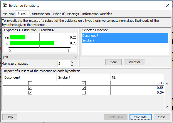
Figure 3: The normalized likelihood (NL) of different subsets of the evidence for the selected state of the hypothesis variable.

Figure 3 shows that the normalized likelihood (NL) of the hypothesis Has bronchitis = yes given on Smoker? is 1.33. This suggests that evidence supports the hypothesis that the patient is suffering from bronchitis (since the normalized likelihood is above one). The evidence on Dyspnoea? is in favor of the alternative hypothesis.

Discrimination

A central question considered by SE analysis is the question of how different subsets of the evidence discriminates between competing hypotheses. The challenge is to compare the impact of subsets of the evidence on competing hypotheses.

We consider the discrimination between two different hypotheses represented as states of two different variables. The discrimination of a pair of competing hypotheses is based on the calculation of Bayes’ factor for all subsets of a selected set of evidence.

\[B = \frac{\text{posterior odds ratio}}{\text{prior odds ratio}} = \frac{P(x | \varepsilon ') / P(y | \varepsilon ')}{P(x) / P(y)} = \frac{P( \varepsilon ' | x)}{P( \varepsilon ' | y)} = \frac{L(x | \varepsilon ')}{L(y | \varepsilon ')}\]

This requires one propagation for each subset.

Using the dialog shown in Figure 4 we may investigate how each subsets of the selected evidence discriminates between two competing hypotheses.

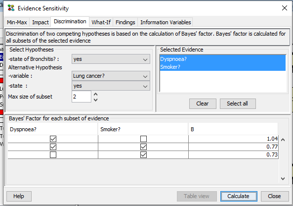
Figure 4: Discrimination between the hypothesis Has bronchitis = true and the alternative hypothesis Has lung cancer = true.

Figure 4 shows Bayes’ factor between the hypothesis Has bronchitis = true and the alternative hypothesis Has lung cancer = true for each subset of the selected evidence. All subsets (except the empty set) support the alternative hypothesis (i.e. that the patient is suffering from lung cancer)

What-If

In what-if SE analysis the type of question considered is the following. What if an observed discrete or continuous random variable had been observed to a value different from the value actually observed. For an observed continuous chance node we consider a limited number of possible values computed based on the mean and standard deviation of the node. The number of values considered for a continuous node is specified by the user as Number of values. This the number of values above and below the mean value, i.e., twice this number of values will be consider plus the mean value.

We consider a hypothesis driven approach to what-if analysis. Hypothesis driven what-if analysis is performed by computing the posterior distribution of the hypothesis variable for each possible state of the observed variable.

Using the dialog shown in Figure 5 we may investigate the consequences of changing the observed state of an evidence variable.

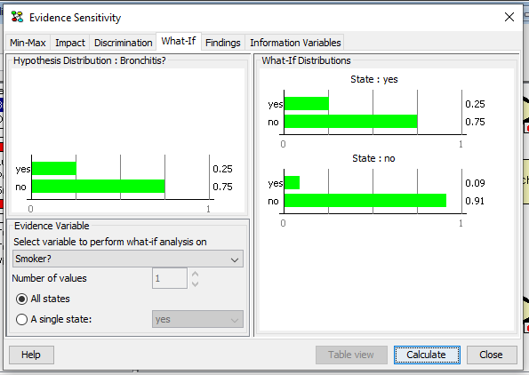
Figure 5: The posterior distribution of the hypothesis variable Has bronchitis has a function of the observed state of Smoker?.

Figure 5 shows how the posterior distribution of the hypothesis variable Has bronchitis changes as a function of the observed state of Smoker?.

Findings

The impact of each finding on the probability of the hypothesis is determined by computing and comparing the prior probability of the hypothesis, the posterior probability of the hypothesis given the entire set of evidence and the posterior probability of the hypothesis given the entire set of evidence except the finding.

The notions of an important finding, a sufficient set of evidence, and a redudant finding are central to findings SE analysis:

• A finding is important when the difference between the probability of the hypothesis given the entire set of evidence except the finding and the probability of the hypothesis given the entire set of evidence is too large.

• A subset of evidence, e.g. the entire set of evidence except a certain finding, is sufficient when the probability of the hypothesis given the subset of evidence is almost equal to the probability of the hypothesis given the entire set of evidence.

• A finding is redundant when the probability of the hypothesis given the entire set of evidence except the finding is almost equal to the probability of the hypothesis given the entire set of evidence.

The impact of each finding may be considered for each state or a certain state of the hypothese variable. Sufficiency and importance thresholds are specified by the user.

Using the dialog shown in Figure 6 and 7 we may investigate the of a finding on the posterior distribution of the hypothesis variable.

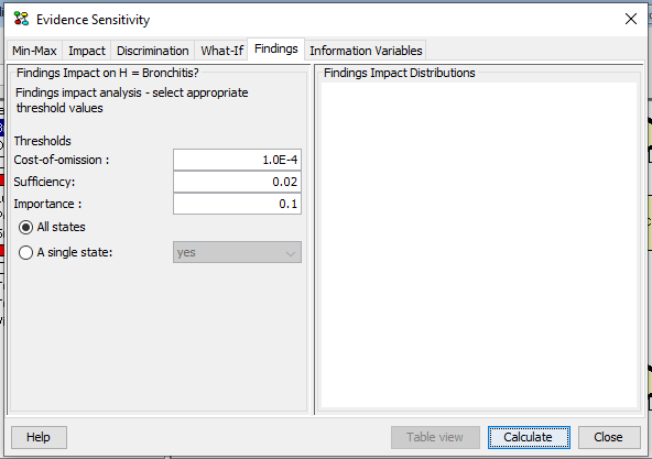
Figure 6: Findings

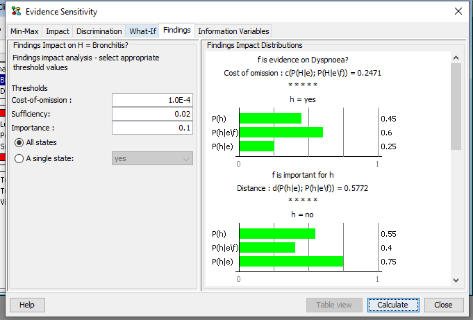
Figure 7: The impact of findings on B.

Figure 6 and 7 illustrates the impact of the finding on Smoker? on the hypothesis Has bronchitis = false (corresponding to H in state false, i.e. h=false).

Information Variables

Min-max SE analysis on a hypothesis variable is performed relative to a set of information variables. The set of information variables can be selected as indicated in Figure 8.

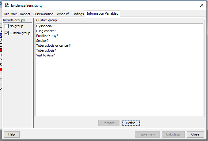
Figure 8: Selecting the set of information variables.

Selecting information variables proceeds in the same way as selecting Target(s) of Instantiations in the d-Separation pane.