Table Generator Tutorial
This tutorial shows you how the Table Generator functionality can be used to simplify the specification of conditional probability tables (CPTs) for discrete chance nodes, utility tables for utility nodes, and initial policies for decision nodes. The tutorial describes how these tables can be described compactly using models and expressions. This is particularly useful when the conditional probability distribution for a variable follows (at least approximately) certain functional or distributional forms. In such cases it is cumbersome to specify the conditional probability table (CPT) manually.
Since the type of expressions available depends on the type of the node, it will be illuminating to discuss the different node sub-types that are supported by the HUGIN Decision Engine.
A model consists of a list of discrete nodes and a set of expressions (one expression for each configuration of the states of the nodes). The list of nodes of a model is referred to as model nodes.
An expression is built using standard statistical distributions (e.g., Normal, Binomial, Beta, Gamma, etc.), arithmetic operators, standard mathematical functions (e.g., logarithmic, exponential, trigonometric, and hyperbolic functions), logical operators (e.g., and, or, if-then-else), and relations (e.g., less-than, equals).
Expressions can be constructed manually (see syntax for expressions) or by the assistance of the Expression Builder, which guides the user through the construction, using series of dialog boxes.
Sub-Typing of Discrete Nodes
The different operators used in an expression have different return types and different type requirements for arguments. Thus, in order to provide a rich language for specifying expressions, it is convenient to have a classification of the discrete chance and decision nodes into different groups (see also section Node Type):
Labelled nodes can be used in equality comparisons and to express deterministic relationships. For example, a labelled node C1 with states “State 1” and “State 2” can appear in an expression like ‘if (C1 == “State 1”, Distribution (0.2, 0.8), Distribution (0.4, 0.6))’ for P(C2 | C1), where C2 is another discrete chance node with two possible states.
Boolean nodes represent the truth values ‘false’ and ‘true’ (in that order) and can be used in logical operators. For example, for a Boolean node, B0, being a the logical OR of its (Boolean) parents, B1, B2, and B3, P(B0|B1, B2, B3) can be specified simply as ‘or (B1, B2, B3)’.
Numbered nodes represent increasing sequences of numbers (integers or reals) and can be used in arithmetic operators, mathematical functions, etc.
Interval nodes represent disjoint intervals on the real line and can be used in the same way as numbered nodes. In addition, they can be used when specifying the intervals over which a continuous quantity are to be discretized.
Numbered nodes and interval nodes are jointly referred to as numeric nodes.
Constant Values
The following kinds of constants can be used in expressions:
State labels (i.e., sequences of characters encapsulated in quotation characters (“)).
Numeric values (including integers, reals, and intervals of integers and reals). For example, a valid numeric expression could be “X + 3.4” (without the quotation characters; otherwise, it will be interpreted as a state label), where X is the name of a numeric node.
Infinity. Positive infinity is denoted by “inf” (without the quotation characters), and negative infinity by “-inf”.
Boolean values: “false” and “true” (without the quotation characters). Notice that the Boolean constants must be indicated using lower case.
Model Nodes
Quite often one needs different expressions depending on the states of one or more parent nodes. Using a number of nested if-then-else expressions is one way of coping with this. The resulting expression, however, often gets very complicated and hence difficult to evaluate by visual inspection and, thus, difficult to maintain.
To simplify complicated expressions, the notion of model nodes can be quite useful.
As mentioned above, a model for a CPT consists of a list of model nodes and an expression for each configuration of the states of the model nodes. That is, if there are no model nodes, the model contains a single expression.
The model nodes for a particular model constitute a subset of the parents of the node to which the model belongs. This subset is specified under the Table tab of the Node Properties dialog box.
An example of the use of model nodes is given in the below example, Discretization of a Random Variable.
Simple Examples
Number of People
Assume that in some application we have probability distributions over the number of males and females, where the distributions are defined over intervals [0 - 100), [100 - 500), [500 - 1000), and that we wish to compute the distribution over the total number of individuals given the two former distributions. It is a simple but tedious task to specify P(NI | NM, NF), where NI, NM, and NF stands for number of individuals, number of males, and number of females, respectively. A much more expedient way of specifying this conditional probability distribution would be to let NM and NF be represented as interval nodes with states [0 - 100), [100 - 500), and [500 - 1000), and to let NI be represented as an interval node with states [0 - 200), [200 - 1000), and [1000 - 2000), for example, and then define P(NI | NM, NF) through the simple expression NI = NM + NF.
To specify that expression, we first select Expressions mode, see the Node Table tutorial. Next, we activate the expression text field by clicking it by the left mouse button. Finally, we type the string “NM + NF” (without the quotation characters), using the keyboard. Figure 1 shows the resulting table for node NI with this expression and the resulting CPT, where the numbers displayed are derived from the expression by selecting menu item “Show as table” from the “Expressions” submenu of the “Functions” menu.
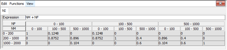
Figure 1: A CPT specified via an expression. The CPT is specified for a discrete chance node NI that has parents NM and NF.
Fair or Fake Die?
As another example, consider the problem of computing the probabilities of getting n 6’s in n rolls with a fair die and a fake die, respectively. A random variable, X, denoting the number of 6’s obtained in n rolls with a fair die is binomially distributed with parameters (n, 1/6). Thus, the probability of getting k 6’s in n rolls with a fair die is P(X = k), where P is a Binomial(n, 1/6). Assuming that for a fake die the probability of getting 6 eyes in one roll is 1/5, the probability of getting k 6’s in n rolls with a fake die is Q(X = k), where Q is a Binomial(n, 1/5).
A Bayesian-network model of this problem is shown in Figure 2, where the node n6s (labeled “# 6’s”) depends on the number of rolls, represented by the node n_rolls (labeled “# rolls”), and on the probability of the die being fake, represented by the node fake_die (labeled “Fake die?”). Now, if we let n_rolls be a numbered node with states 1, 2, 3, 4, 5, let fake_die be a boolean node, and let n6s be a numbered node with states 0, 1, 2, 3, 4, 5, then P(n6s | n_rolls, fake_die) can be specified very elegantly using the expression P(n6s | n_rolls, fake_die) = Binomial (n_rolls, if (fake_die, 1/5, 1/6)).
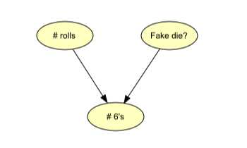
Figure 2: A Bayesian-network model for the fake die problem.
To specify that expression, we may proceed as in the Number of People example or we may wish to use the Expression Builder (activated by selecting the “Build Expression” item of the “Expressions” submenu of the “Functions” menu) . The result of the specification and the derived probabilities are shown in Figure 3.
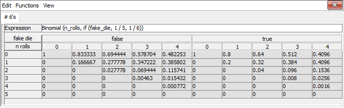
Figure 3: The CPT for the fake die problem specified very compactly using a simple expression.
Notice that we could equivalently specify P(n6s | n_rolls, fake_die) = if (fake_die, Binomial (n_rolls, 1/5), Binomial(n_rolls, 1/6)).
Discretization of a Random Variable
Assume that P(C1 | C2) can be approximated by a Normal distribution with mean given by C2 and with variance 1, where C2 is an interval variable with states [-5,-1), [-1,0), [0,1), [1,5). If the discretization of C1 given by the intervals [-infinity,-5), [-5,-2), [-2,0), [0,2), [2,5), [5,infinity) is found to be suitable, then we can specify P(C1 | C2) simply as Normal(C2, 1), see Figure 4.
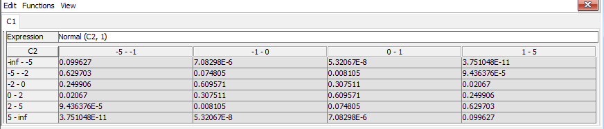
Figure 4: The CPT for variable C1 specified through discretization of a Normal distribution with mean given by the (interval) parent variable C2 and with variance 1.
If, in addition, C1 has another parent, say C3, which is a labelled node with states, say, “State 1” and “State 2” and that the variance of the Normal distribution is 1 if C3 is in state “State 1” and 1.5 if C3 is in state “State 2”, then we can define C3 as a so-called model node, which allows us to specify different expressions for the different states of C3, see Figure 5.
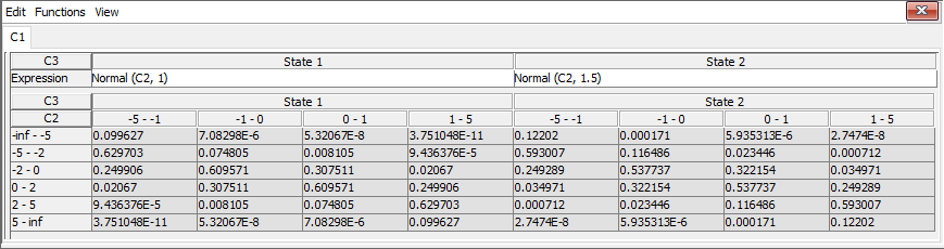
Figure 5: Similar to Figure 4, except that C1 has got a new parent, C3, defined as a model node, allowing the specification of different expressions for the different states of C3.
Notice that the use of model nodes is not strictly necessary, as we can alternatively condition on the states of the (model) node(s). The use of model nodes, however, often makes the specification much less cluttered and easier to read and maintain. For example, if we don’t specify C3 as a model node, P(C1 | C2, C3) can be specified through the expression P(C1 | C2, C3) = if (C3 == “State 1”, Normal (C2, 1), Normal (C2, 1.5)), see Figure 6.
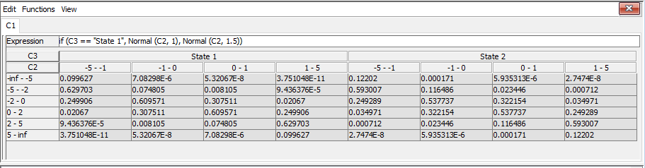
Figure 6: Similar to Figure 5, except that instead of specifying C3 as a model node the two expressions are merged into one expression, where we condition on the states of C3.
Operators and Functions
The basic operators and functions available for composing expressions are list below.
Binary Numeric Operators
The following binary (infix) operators can be applied to numeric expressions.
+ (addition)
- (subtraction)
* (multiplication)
/ (division)
^ (power)
Examples:
C1 + C2
C1 ^ 3
where C1 and C2 are numeric nodes (i.e., numbered nodes and/or interval nodes).
Unary Numeric Operators
An numeric expression can be negated using the unary negation operator:
- (negation)
Binary Comparison Operators
The following binary (infix) operators can be used for comparing labels (i.e., strings), numbers, and Booleans (both operands must be of the same type). Only the equality operators (i.e., = and !=) may be applied to labels and Boolean expressions. Each of the operators returns a Boolean value.
= (equals)
== (equals)
!= (not equals)
<> (not equals)
< (less than)
> (greater than)
<= (less than or equals)
>= (greater than or equals)
Examples:
C1 == C2
C1 > 5
where C1 and C2 are numeric nodes (i.e., numbered nodes and/or interval nodes).
Min and Max Functions
The following functions compute the minimum or maximum of a list of numeric expressions.
min(x1, x2, …, xn) returns the minimum of the argument expressions.
max(x1, x2, …, xn) returns the maximum of the argument expressions.
Examples:
min(C1, C2, 10)
max(min(C1, C2, 10), max(C3, C4))
where C1, …, C4 are numeric nodes (i.e., numbered nodes and/or interval nodes).
Standard Mathematical Functions
The following list contains standard mathematical functions, which can be applied to a single numeric expression.
log(x) returns the natural (i.e., base e) logarithm to x.
log2(x) returns the base 2 logarithm to x.
log10(x) returns the base 10 logarithm to x.
exp(x) returns the exponential to x (i.e., e^x).
sin(x) returns the sine of x.
cos(x) returns the cosine of x.
tan(x) returns the tangent of x.
sinh(x) returns the hyperbolic sine of x.
cosh(x) returns the hyperbolic cosine of x.
tanh(x) returns the hyperbolic tangent of x.
sqrt(x) returns square root of x.
abs(x) returns the absolute value of x.
Examples:
log(C1)
abs(sin(C1))
where C1 is a numeric node (i.e., a numbered node or an interval node).
Floor and Ceiling Functions
The floor and ceiling functions round the result of real numeric expressions to integers.
floor(x) returns the greatest integer less than or equal to x.
ceil(x) returns the smallest integer greater than or equal to x.
Examples:
floor(C1 * C2)
ceil(C1 ^ 2)
where C1 and C2 are numeric nodes (i.e., numbered nodes and/or interval nodes).
Modulo Function
The modulo function gives the remainder of a division of two numeric expressions. Of course, the divisor expression must be non-zero.
mod(x,y) returns x - y * floor(x / y), where x and y can be arbitrary real numbers with y != 0.
Example:
mod(C1, C2 ^ 2)
where C1 and C2 are numeric nodes (i.e., numbered nodes and/or interval nodes).
If-Then-Else
Conditional expression (with three arguments) can be specified:
if(px, tx, fx), where px must be a Boolean expression, and the second and third arguments must have the same type. If px evaluates to ‘true’, the value of expression tx is returned; otherwise, the value of expression fx is returned. The type of the if-expression is the type of tx and fx.
Examples:
if(FakeDie, Binomial(n, 1/2), Binomial(n, 1/6))
if(C1 == C2, Distribution(1, 2), Distribution(1, 3))
where FakeDie is a Boolean node, n is a numeric node, and C1 and C2 are nodes of arbitrary (but identical) type.
Logical Operators
The following standard logical operators are available. They all take Boolean expressions as arguments.
and(x1, x2, …, xn) returns ‘true’ if all argument expressions evaluate to ‘true’.
or(x1, x2, …, xn) returns ‘true’ if at least one of the argument expressions evaluate to ‘true’.
not(x) returns ‘true’ if x evaluates to ‘false’; otherwise, returns ‘false’.
The evaluation of the argument expressions of ‘and’ is done sequentially, and the evaluation terminates whenever an argument evaluates to ‘false’. Similarly, the evaluation of the argument expressions of ‘or’ terminates whenever an argument evaluates to ‘true’.
Example:
and(C1, or(C2, not(C3)))
where C1, C2 and C3 are Boolean nodes.
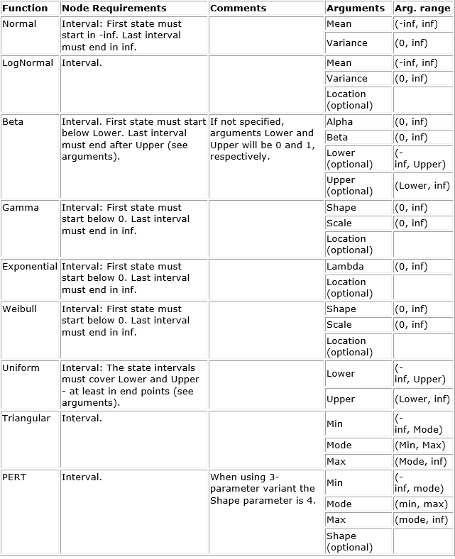
Continuous Statistical Distributions
A number of continuous statistical distributions are available. See Continuous Distributions for details.
Normal
LogNormal
Beta
Gamma
Exponential
Weibull
Uniform
Triangular
PERT
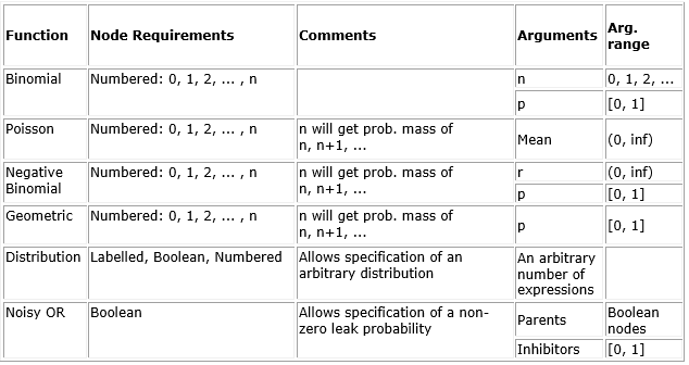
Discrete Statistical Distributions
A number of discrete statistical distributions are available. See Discrete Distributions for details.
Binomial
Poisson
Negative Binomial
Geometric
Distribution
Noisy OR
Statistical Distributions
Continuous Distributions
The following continuous distribution functions are available for interval nodes only.
Example:
Normal(C1, C2) - specifies the conditional probabilities for an interval node from a Normal distribution with mean given by the value of the numeric parent node C1 and variance given by another numeric parent node C2.
Truncation operator:
In addition a truncation operator can be applied to a continuous statistical distribution in order to form a truncated distribution. The operator takes either two or three arguments. When three arguments are specified, the first and third arguments must be numeric expressions denoting, respectively, the left and right truncation points, while the second argument must denote the distribution to be truncated. Either the first or the third argument can be omitted. Omitting the first argument results in a right-truncated distribution, and omitting the third argument results in a left-truncated distribution.
Example:
truncate (-4, Normal (0, 1), 4) - specification of a truncated normal distribution. The distribution is truncated at the left at -4 and at the right at 4.
truncate (4, Normal (0, 1)) - A left truncated (at -4) normal distribution.
Discrete Distributions
A variety of discrete distribution functions can be specified. There are four standard statistical distribution functions, which all must be specified for numeric nodes. The special function called ‘Distribution’ allows one to specify arbitrary distribution functions, where an expression must be specified for each possible outcome of the variable in question.
Examples:
Binomial(4, 0.2)
NegativeBinomial(sqrt(10), 0.4)
NoisyOR(C1, 0.1, C2, 0.05, true, 1) - specifies that a Boolean effect node is ‘true’ with probability 1 - 0.1 if the Boolean cause (parent) node C1 is ‘true’ and C2 is ‘false’, 1 - 0.05 if the Boolean cause (parent) node C2 is ‘true’ and C1 is ‘false’, and 1 - 0.1*0.05 if both C1 and C2 are ‘true’. Further, it specifies that the effect node is ‘false’ with probability 1 if both C1 and C2 are ‘false’ (i.e., a leak probability of zero has been specified in this example).
Distribution(if(C1 = “State 1”, 3, 5), 2) - specifies the distribution for a binary node with a Labelled parent node C1.
Syntax for Expressions
<Expression> ::= <Simple expression> <Comparison> <Simple expression> |

             <Simple expression>


<Simple expression> ::= <Simple expression> <Plus or minus> <Term> |
                    <Plus or minus> <Term> |
                    <Term>

<Term> ::= <Term> <Times or divide> <Exp factor> |
               <Exp factor>

<Exp factor> ::= <Factor> ^ <Exp factor> |
                                 <Factor>


<Factor> ::= <Unsigned number> |
                 <Node name> |
                 <String> |
                 false |
                 true |
                 (<Expression>) |
                 <Operator> (<Expression sequence>)


<Expression sequence> ::= <Empty> | <Expression> [, <Expression>]*

<Comparison> ::= == | = | != | <> | < | <= | > | >=

<Plus or minus> ::= + | -

<Times or divide> ::= * | /

<Operator> ::= truncate | Normal | LogNormal | Beta | Gamma | Exponential | Weibull | Uniform | Triangular | PERT
       Binomial | Poisson | NegativeBinomial | Geometric | Distribution |
       NoisyOR | min | max | log | log2 | log10 | exp |
       sin | cos | tan | sinh | cosh | tanh |
       sqrt | abs | floor | ceil | mod |
       if | and | or | not