Bayesian Network Technology in the HUGIN Development Environment
This text provides you with an overview of Bayesian networks, LIMID models, and networks with conditional Gaussian variables (also known as Bayesian networks). More detailed information on these and other issues can be found in specialized sections and tutorials
Probabilistic graphical models (of which Bayesian networks and LIMIDs are excellent examples) are especially suitable for domains with inherent uncertainty. Domain models based on Bayesian network technology can be built using the HUGIN Graphical User Interface, an easy-to-use graphical user interface built on top of the Java API provided with the HUGIN Developer package. Stand-alone applications using network technology can be built using the HUGIN APIs, a series of C, C++, and Java libraries and an ActiveX server providing access to the facilities of the HUGIN Decision Engine (HDE) for the application programmer.
Bayesian Networks
Bayesian networks are often used to model domains that are characterized by inherent uncertainty. (This uncertainty can be due to imperfect understanding of the domain, incomplete knowledge of the state of the domain at the time where a given task is to be performed, randomness in the mechanisms governing the behavior of the domain, or a combination of these.)
Formally, a Bayesian network can be defined as follows:
Definition (Bayesian Network) A Bayesian network is a directed acyclic graph with the following properties:
Each node represents a random variable.
Each node representing a variable A with parent nodes representing variables B1, B22,…, Bn is assigned a conditional probability table (CPT):
The nodes represent random variables, and the edges represent probabilistic dependences between variables. These dependences are quantified through a set of conditional probability tables (CPTs): Each variable is assigned a CPT of the variable given its parents. For variables without parents, this is an unconditional (also called a marginal) distribution.
Example 1
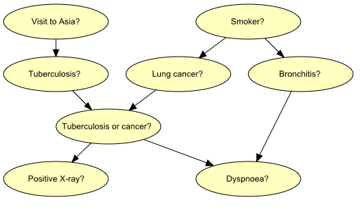
Figure 1: Graph representing structural aspects of medical knowledge concerning lung diseases.
Figure 1 shows a model for the following piece of fictitious medical knowledge:
“Shortness-of-breath (dyspnoea) [d] may be due to tuberculosis [t], lung cancer [l] or bronchitis [b], or none of them, or more than one of them. A recent visit to Asia [a] increases the risk of tuberculosis, while smoking [s] is known to be a risk factor for both lung cancer and bronchitis. The result of a single chest X-ray [x] does not discriminate between lung cancer and tuberculosis, neither does the presence or absence of dyspnoea” (Lauritzen & Spiegelhalter 1988).
The last fact is represented in the graph by the intermediate variable e. This variable is a logical-or of its two parents (t and l); it summarizes the presence of one or both diseases or the absence of both.
An important concept for Bayesian networks is conditional independence. Two sets of variables, A and B, are said to be (conditionally) independent given a third set C of variables if when the values of the variables C are known, knowledge about the values of the variables B provides no further information about the values of the variables A:
Conditional independence can be directly read from the graph as follows: Let A, B, and C be disjoint sets of variables, then
identify the smallest sub-graph that contains A B C and their ancestors;
add undirected edges between nodes having a common child;
drop directions on all directed edges.
Now, if every path from a variable in A to a variable in B contains a variable in C, then A is conditionally independent of B given C (Lauritzen et al. 1990).
Example 2
If we learn the fact that a patient is a smoker, we will adjust our beliefs (increased risks) regarding lung cancer and bronchitis. However, our beliefs regarding tuberculosis are unchanged (i.e., t is conditionally independent of s given the empty set of variables). Now, suppose we get a positive X-ray result for the patient. This will affect our beliefs regarding tuberculosis and lung cancer, but not our beliefs regarding bronchitis (i.e., b is conditionally independent of x given s). However, had we also known that the patient suffers from shortness-of-breath, the X-ray result would also have affected our beliefs regarding bronchitis (i.e., b is not conditionally independent of x given s and d).
These (in)dependences can all be read from the graph of Figure 1 using the method described above.
Another, equivalent and very popular criterion for reading statements of conditional independence is d-separation (Pearl 1988).
Inference
Inference in a Bayesian network means computing the conditional probability for some variables given information (evidence) on other variables. This is easy when all available evidence is on variables that are ancestors of the variable(s) of interest. But when evidence is available on a descendant of the variable(s) of interest, we have to perform inference opposite the direction of the edges. To this end, we employ Bayes’ Theorem:
HUGIN inference is essentially a clever application of Bayes’ Theorem; details can be found in the paper by Jensen et al. (1990(1)).
Limited Memory Influence Diagrams
A LIMID is a Bayesian network augmented with decision and utility nodes (the random variables of a LIMID diagram are often called chance variables). Edges into decision nodes indicate time precedence: an edge from a random variable to a decision variable indicates that the value of the random variable is known when the decision will be taken, and an edge from one decision variable to another indicates the chronological ordering of the corresponding decisions. The network must be acyclic.
We are interested in making the best possible decisions for our application. We therefore associate utilities with the state configurations of the network. These utilities are represented by utility nodes. Each utility node has a utility function that to each configuration of states of its parents associates a utility. (Utility nodes do not have children). By making decisions, we influence the probabilities of the configurations of the network. We can therefore compute the expected utility of each decision alternative (the global utility function is the sum of all the local utility functions). We shall choose the alternative with the highest expected utility; this is known as the maximum expected utility principle.
When we have observed the values of the variables that are parents of the first decision node in the LIMID, we want to know the maximum expected utilities for the alternatives of this decision. The HUGIN Decision Engine will compute these utilities on the assumption that all future decisions will be made in an optimal manner (using all available evidence at the time of each decision). Similar considerations also apply to the remaining decisions.
The computational method underlying the implementation of LIMIDs in the HUGIN Decision Engine is described by S. L. Lauritzen and D. Nilsson (2001).
Example 3
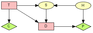
Figure 2: LIMID model for the oil wildcatters decision problem: T represents the decision whether or not to test; D represents the decision whether to drill or not to drill; S represents the outcome of the seismic soundings test (if the oil wildcatter decides to test); H represents the state of the hole; C represents the cost associated with the seismic soundings test; and P represents the expected payoff associated with drilling.
An oil wildcatter must decide whether or not to drill. He is uncertain whether the hole is dry, wet, or soaking. At a cost of $10,000, the oil wildcatter could take seismic soundings which will help determine the underlying geological structure at the site. The soundings will disclose whether the terrain below has closed structure (good), open structure (so-so), or no structure (bad).
The cost of drilling is $70,000. If the oil wildcatter decides to drill, the expected payoff (i.e., the value of the oil found minus the cost of drilling) is $-70,000 if the hole is dry, $50,000 if the hole is wet, and $200,000 if the hole is soaking; if the oil wildcatter decides not to drill, the payoff is (of course) $0.
The experts have estimated the following probability distribution for the state of the hole: P(dry)=0.5, P(wet)=0.3, and P(soaking)=0.2. Moreover, the seismic soundings test is not perfect; the conditional probabilities for the outcomes of the test given the state of the hole are:
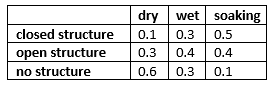
Figure 3: CPT for the outcomes of the test
Figure 2 shows LIMID model for the oil wildcatters decision problem. Random variables are depicted as circles, decision variables are depicted as squares, and utilities are depicted as diamonds.
On the basis of this LIMID, the HUGIN Decision Engine computes the utility associated with testing to be $22,500 and the utility associated with not testing to be $20,000. So the optimal strategy is to perform the seismic soundings test, and then decide whether to drill or not to drill based on the outcome of the test.
[This example is due to Raiffa (1968). A more thorough description of this example is found in the Examples section.]
Networks with Conditional Gaussian Variables
The HUGIN Decision Engine is able to handle networks with both discrete and continuous random variables. The continuous random variables must have a Gaussian (also known as a normal) distribution conditional on the values of the parents.
The distribution for a continuous variable Y with discrete parents I and continuous parents Z is a (one-dimensional) Gaussian distribution conditional on the values of the parents:
Note that the mean depends linearly on the continuous parent variables and that the variance does not depend on the continuous parent variables. However, both the linear function and the variance are allowed to depend on the discrete parent variables. These restrictions ensure that exact inference is possible.
Note that discrete variables cannot have continuous parents.
Example 4
Figure 3 shows a network model for a waste incinerator (Lauritzen 1992):
“The emissions (of dust and heavy metals) from a waste incinerator differ because of compositional differences in incoming waste [W]. Another important factor is the waste burning regimen [B], which can be monitored by measuring the concentration of CO2 in the emissions [C]. The filter efficiency [E] depends on the technical state [F] of the electrofilter and on the amount and composition of waste [W]. The emission of heavy metals [M:sub:`o`] depends on both the concentration of metals [M:sub:`i`] in the incoming waste and the emission of dust particulates [D] in general. The emission of dust [D] is monitored through measuring the penetrability of light [L].”
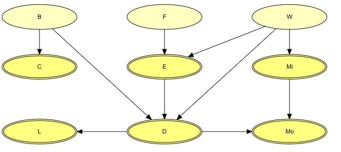
Figure 3: The structural aspects of the waste incinerator model: B, F, and W are discrete variables, while the remaining variables are continuous.
The result of inference within a network model containing conditional Gaussian variables is - as always - the beliefs (i.e., marginal distributions) of the individual variables given evidence. For a discrete variable this amounts to a probability distribution over the states of the variable. For a conditional Gaussian variable two measures are provided:
the mean and variance of the distribution;
since the distribution is in general not a simple Gaussian distribution, but a mixture (i.e., a weighted sum) of Gaussians, a list of the parameters (weight, mean, and variance) for each of the Gaussians is available.
Example 5
From the network shown in Figure 3 (and given that the discrete variables B, F, and W are all binary), we see that
the distribution for C can be comprised of up to two Gaussians (one if B is instantiated);
initially (i.e., with no evidence incorporated), the distribution for E is comprised of up to four Gaussians;
if L is instantiated (and none of B, F, or W is instantiated), then the distribution for E is comprised of up to eight Gaussians.