Correlation Analysis Dialog

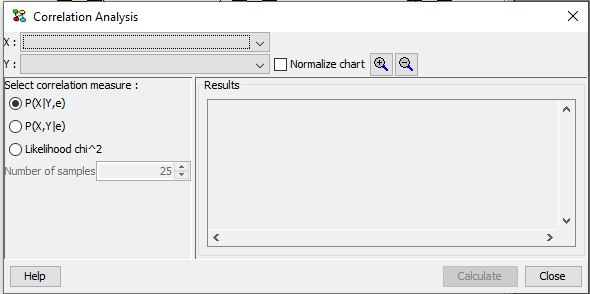
Figure 1 shows the correlation analysis dialog as it appears after being activated. In dialog the correlation between a pair of discrete chance node can be analysed using a number of different measures.

Figure 1: The Correlation Analysis Dialog.

The dialog supports three different methods for analysing the correlation between a pair of nodes X and Y: the conditional probabability distribution, the joint probability distribution, and the Pearson test.

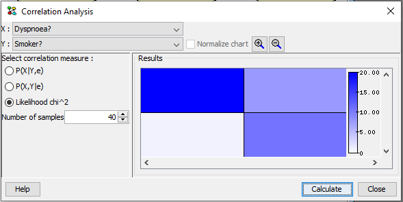
The correlation between the selected pair of nodes X and Y is illustrated using a color intensity chart. Each entry of the chart corresponds to a configuration of X and Y. The more intense the color is the higher the value displayed in the entry is. The entries of the color chart are computed using the selected correlation measure when the user press Compute.

If the normalize chart check box is checked, then the numbers displayed in the color chart are normalized such that the maximum value has the maximum color intensity. This is useful, for instance, if the values in the joint probability distribution are all much less than one. In this case the color intensity will be low. By normalizing the chart, the maximum value will have maximum color intensity.

In the following sections the three methods for analysing the correlation between a pair of discrete chance variables are described.

Conditional Probability

Figure 2 shows the conditional probability distribution of X given Y computed based on the entered and propagated evidence.

Figure 2: The conditional probability distribution of X given Y.

Notice that X and Y can in principle be any pair of discrete chance nodes in the model.

The computation of the conditional probability distribution may in principle fail with an out-of-memory error. This will happen if the tables in the underlying junction tree become too large during the process of computing the conditional.

Joint Probability Distribution

Figure 3 shows the joint probability distribution of X and Y computed based on the entered and propagated evidence.

Figure 3: The joint probability distribution over X and Y.

Notice that X and Y can in principle be any pair of discrete chance nodes in the model. The computation of the joint probability distribution may in principle fail with an out-of-memory error. This will happen if the tables in the underlying junction tree become too large during the process of computing the joint.

Pearson Test

Figure 4 shows the joint counts table X and Y computed based on the entered and propagated evidence.

Figure 4: A table of counts over X and Y.

The table of counts is computed by generating a sample over X and Y consisting of the number of samples defined by the user. The sample is generated based on the evidence entered and propagated in the network. Based on this sample the likelihood chi² score is computed and displayed for each configuration of X and Y.