Introduction

This document describes how to build a (limited-memory) influence diagram (LIMID) to model a simplified version of the dice game called “Tænkeboks”. The objective of this modeling is to find a winning strategy against a presumed strategy of the opponent. The influence diagram is designed and afterwards implemented in HUGIN. Finally this implementation is used to determine an optimal counter strategy against the opponent’s presumed strategy.

This document has been written by Michael Höhle with the support of Søren Andersen, Lisa Elgaard, Brian Jensen, Brian Kristiansen and Søren Mogensen. The network and it’s documentation originate from a DAT3 (7th semester) project worked out by group C1-213 at Department of Computer Science, Aalborg University, in the fall of 1997. The supervisor of the DAT3 project was Dennis Nilsson.

The Simplified Tænkeboks

Consider the following simplified version of the dice game Tænkeboks. Two players named Arne and Bente (typical Danish names) participate in the game. Each player holds a two sided die (with the labels “1” and “2”).

Initially both players roll their die without showing the result to each other. The goal of the game is to guess how many identical die values are present based upon knowledge of one’s own die. The following bids are possible:

• 1 (at least one “1”),

• 2 (at least one “2”),

• 2·1 (both dice show “1”),

• 2·2 (both dice show “2”).

Assume Arne starts the game. He has to choose between one of the above 4 bids. After Arne’s bid, Bente has to decide whether to believe in Arne’s bid and hence bid up or to call. If Bente doesn’t call it is Arne’s turn to consider Bente’s last bid. The game continues until one of the players decides to call. A call results in both players revealing their die thus resolving whether the bid which was called upon was present on the table or not. This process determines winner and loser of the game.

Influence Diagrams and the Simplified Tænkeboks

Imagine that one foggy night at the pub you convince your best friend Arne to play some rounds of the above game. To make things more interesting the loser of each game has to buy the next round of beer. What is a good strategy for Bente?

There are several approaches e.g. one could analyze the above game by game theoretic methods or one could try to use influence diagrams. Since game theory tends to be quite complex and cumbersome we shall concentrate on the latter.

Based on an estimate of Arne’s strategy we will solve the influence diagram in order to find an optimal counter strategy. The key problem is how to make a good estimate of Arne’s strategy. We assume that you have been playing quite a lot of games of simple Tænkeboks against Arne and hereby achieved a pretty good understanding of his strategy.

An Influence Diagram for Simple Tænkeboks Implemented in HUGIN

For the sake of simplicity we assume from now on that Arne always is in the lead, i.e., he always is the first to bid in a game.

Determining the Chance and Decision Variables

Initially we need to find out which chance and decision variables we need and which states they should have. A prudent way to obtain this is to find the actors in our game and the actions they can perform.

By analyzing the maximal sequence of bids in one game we determine the maximum amount of bids for each player.

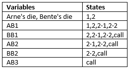
Arne: 1, Bente: 2, Arne: 2·1, Bente: 2·2, Arne: call

Arne has a maximum of three bids during one game. Bente’s maximum is two bids.

Every action is now converted into either a chance variable or a decision variable according to the following rule: If the action is a decision which has to be made by the decision maker it is converted into a decision variable, otherwise it becomes a chance variable. The result is:

Note

the variable “Bente’s die” which corresponds to the result of Bente rolling her die becomes a chance variable, since Bente has no influence on the result of rolling the die.

After finding the variables for our influence diagram it is time to consider which states they should have. The states of the die-variables represent the outcome of rolling a die, whereas the states of the bid-variable reflect the possible bids at the point of the bid-variable. Note how the number of states is based on the maximum bid sequence.

Causal and Information Dependences

The next task is to establish the dependences - represented by links - between the found variables. Our objective with the links is twofold:

• The links indicate the progress of the game

• a link into one of player X’s bid-variables reflects the following: X’s bidding strategy is based on information about the state of the variable from which the link comes.

Experience from playing simple Tænkeboks tells us that when bidding you usually only consider your own dice and the opponent’s last bid. The two objectives and the above experience result in the following diagram shown in Figure 1.

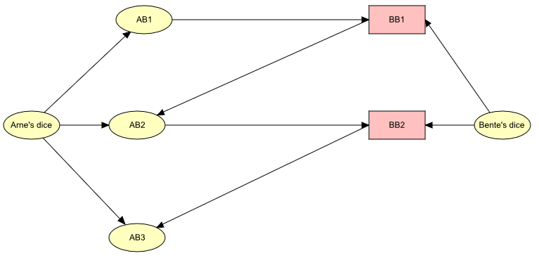
Figure 1: The chance variables and decision variables in the influence diagram together with their dependences.

Note

Arne’s strategy on his first bid only depends on the value of his die. We don’t exactly know his strategy, but we will use our best guess.

The Utility Functions

After introducing the decision variables it is also necessary to add utility functions which determine the outcome of taking a decision. Our utility functions have two goals

1. To determine whether Bente wins or loses once a player calls.

2. To ensure that Bente only performs valid actions (e.g. restrict bidding 1 after Arne bid 2)

The resulting diagram with all the utilities is displayed in Figure 2. To ensure item 1 utility functions are placed between consecutive bids (e.g. U5 between BB1 and AB2). These functions are connected to both the consecutive bid variables and the 2 die variables. All this information is necessary in order to check if the latter bid was a call and if so whether the bid before the call was present or not. This step result in the utility functions U4,U5,U6 and U7. Item 2 is achieved by putting utility functions between AB1 and BB1 (U1) as well as between AB2 and BB2 (U2). Later when assigning values to the utility functions all the illegal actions will be assigned very low values.

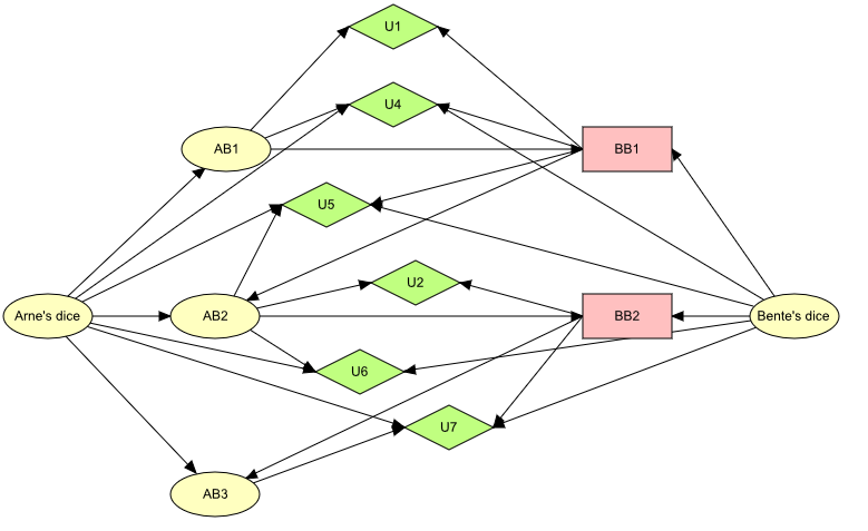
Figure 2: Influence diagram for our model. U1 and U2 guarantee that Bente’s bids are valid and U4, U5, U6, and U7 determine whether Bente wins or not.

Since U1’s set of parents is a subset of U4’s parents the two can be combined in an additive way. This simply means that U1’s utility values are added to U4’s values in the appropriate columns of U4. Similarly U2 and U6 are combined. The resulting influence diagram is displayed in Figure 3.

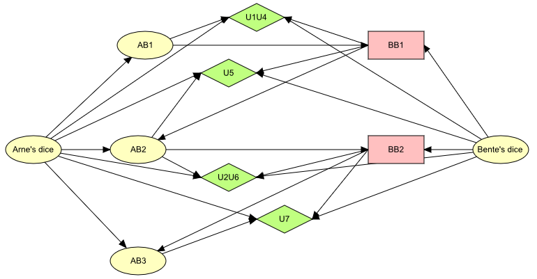
Figure 3: The final influence diagram modeling simple Tænkeboks. Notice how the utility functions have been combined.

Assigning Probabilities and Utility Functions to the Variables

After determining the variables, functions, and their dependences it is necessary to assign the conditional probabilities to the chance variables and utility values to the utility functions. This task can be divided into three subtasks. The gory details of the exact tables implemented in HUGIN are not that important, but are included should you become curious.

1. Assigning probabilities to the two die variables. [Gory details]

2. Assigning conditional probabilities to Arne’s bid variables depending on our estimate of his strategy.

To accomplish this task we need a good guess of Arne’s strategy. To keep things simple we assume that he is following the pretty reasonable deterministic strategy:

• When starting he bids what his die shows. Hereby his bid will always be present on the table.

• If Bente bids 2 and he rolls “1” then he calls.

• If Bente bids 2 and he rolls “2” then he bids 2·2.

• If Bente bids 2·1 or 2·2 he always calls.

In a real game it is more likely that Arne will follow a non-deterministic strategy to conceal his real strategy. Once you get the hang of how the optimal counter strategy is found you can use the influence diagram straight away to find counter strategies against non-deterministic strategies as well. [Gory details] 3. Assigning values to the utility functions so they fulfill the demands from the preceding section. [Gory details]

Finding the Optimal Strategy

We are ready to use the influence diagram to find an optimal counter strategy for Bente against Arne’s strategy.

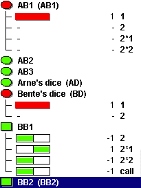
Figure 4: Screenshot from HUGIN where the evidence BD=1 and AB1=1 was entered and since sum-propagated. The action 2·1 in BB1 has the highest expected utility (expected utility = 1).

The following algorithm in HUGIN gives us the desired result:

1. Initialize the network

2. For each state X of Bente’s die variable do

   1. enter X as 100% evidence (click on X in run-mode)

   2. For each possible state Y of Arne’s AB1 variable do

      1. enter Y as 100% evidence (click on Y in run-mode)

      2. sum propagate

      3. The best bid for Bente in BB1 is the action in BB1 with the highest expected utility. (see Figure 4)

In step 2.1 we only loop through the possible states of AB1. With Arne’s strategy it is for example impossible that Arne bids 2·1 in AB1.

Had the game been longer it would have been necessary to insert the optimal action in BB1 as evidence and loop through the states in AB2 in order to determine the optimal action in BB2. But since Bente never really gets to bid a second time this step isn’t included in the algorithm.

By applying this algorithm the following counter strategy for Bente is determined:

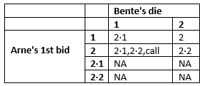
For example, if Bente rolls 2 and Arne bids 2 in his first bid then the strategy tells Bente to bid 2·2. In the situation where Bente rolls a 1 and Arne bids 2 three actions are equally good: 2·1,2·2 and call. To get a deterministic strategy it is sufficient to simply pick one of the possibilities. The NA’s in the table symbolize that a situation cannot occur with Arne’s choice of strategy. All of Bente’s choices are therefore equally good.

The question is how good this counter strategy actually is. By simulating games between the two strategies in the four possible configurations of the dice ([AD=1 and BD=1], [AD=1 and BD=2], [AD=2 and BD=1] or [AD=2 and BD=2]) it becomes obvious that Bente will win 75% of the games! In other words, out of 12 rounds of beer Bente (you) will only have to pay for the 3 while Arne will have to pay for 9. Cheers!

Conclusion

An influence diagram to model a simple version of the game Tænkeboks was designed and since implemented in HUGIN. The resulting diagram is displayed in Figure 3 and the HUGIN implementation can be downloaded from the HUGIN networks page.

Arne’s strategy was guessed and entered into the tables of the diagram. Using HUGIN to enter evidence and propagate, an optimal counter strategy for Bente was found where she could win 75% of the games.

Perspectives

A game theoretic analysis of the game reveals that the strategy assumed for Arne is not a very good one. He could e.g. prefer a strategy where he always bids 2·(whatever he rolled). Hereby he is certain to win 50% of the games - even against Bente’s counter strategy found with the influence diagram! (Game theoretic note: The mentioned strategy combination forms a Nash-equilibrium where both players receive a payoff of zero.)

The assumption that Arne follows a deterministic strategy is pretty unlikely. By changing the values in the tables of Arne’s bid variables Arne can easily be modified to play with a randomized strategy. The algorithm described above also works to find a deterministic counter strategy against Arne’s randomized strategy.

Simple Tænkeboks is quite a boring game. Possible enhancements to increase the joy could be: more sides on your die, more dice per player, a notion of jokers, or even extra players. The problem is that even small enhancements make the complexity of the influence diagram explode.

This network has been installed on your computer with the HUGIN software. Open the network in the HUGIN Graphical User Interface (Note: not all browsers can open HUGIN directly). You can find the network in the directory where you installed HUGIN (e.g. C:Program FilesHuginHugin LiteSamples). You can also find the samples at the HUGIN download area.