Gaussian (Normal) Distribution Function
Continuous chance nodes in a HUGIN network can be specified to have a Gaussian (or normal) distribution function. This text does not cover a mathematically description of the Gaussian distribution function; it only describes how it can be used in HUGIN network nodes.
The Gaussian distribution function is defined on the complete real axis. Any Gaussian distribution function can be specified by its mean and variance parameter. In HUGIN, a continuous chance node can have a single Gaussian distribution function for each configuration of its discrete parents states (both discrete chance nodes and decision nodes). If a continuous chance node has one or more continuous chance node parents, the mean can be linearly dependent on the states of these continuous parents.
In general, the distribution for a continuous variable Y with discrete parents I and continuous parents Z is a (one-dimensional) Gaussian distribution conditional on the values of the parents:
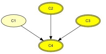
Figure 1 shows an example of the specification of a Gaussian distribution function of a continuous chance node (C4) having one discrete chance node (C1) and two continuous chance nodes (C2 and C3) as parents.

Figure 1: An example of a network where the continuous chance node C4 has one discrete chance node (C1) and two continuous chance nodes (C2 and C3) as parents.

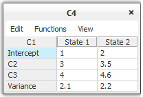
Figure 2: The specification of a Gaussian distribution function for C4 that has one discrete chance node (C1) and two continuous chance nodes (C2 and C3) as parents.
This specification gives a conditional Gaussian distribution function for each of the states of C1 (where N(m,v) is the Gaussian distribution function with mean m and variance v):
P(C4 | C1=”State 1”, C2 = x, C3 = y) = N(1 + 3x + 4y, 2.1)
P(C4 | C1=”State 2”, C2 = x, C3 = y) = N(2 + 3.5x + 4.6y, 2.2)
The mean of each distribution function for C4 is thus a sum of a specified mean parameter and a weighted sum over the values of the continuous parents, where the weights are given by the numeric values in the C2 and the C3 rows of the table in Figure 2.
Only the mean depends linearly on the continuous parent nodes. The variance is constant for each configuration of the states of the discrete parents.
See Introduction to Bayesian Networks for an example of the modeling of a real-world problem involving several discrete and continuous variables.