Data Frame

HUGIN can load a data file as a project frame, the data frame. Data files can be inspected, manipulated and analyzed as the contents of the data frame is a data matrix with additional functionallity for performing batch propagation in run mode models.

To open a new data frame and load a data file, click in the menu of the main HUGIN frame File -> Open Data File and select a data file.

Figure 1: Typical data frame - A data frame containing a data file for the chest clinic model with only symptom observations.

To configure a data frame for batch propagation, we must first load a network model and set the model to run mode (Note. batch propagation functionallity is only available for models in run-mode!).

Then in the data frame, click the Model menu and then click Select a Run-Mode Model. A dialog appears, containing all the current project frames to pick from.

Figure 2: Pick a project for doing batch propagation.

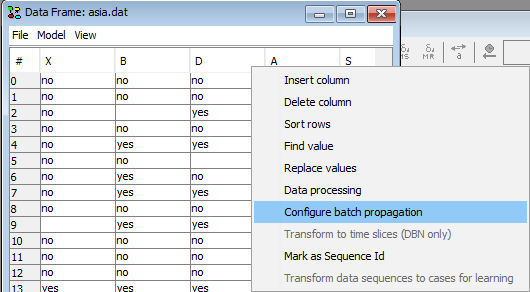
When a run mode model has been configured for the data frame, we can configure the batch propagation options. To do this, right click a column header in the data matrix and select the Configure batch propagation option.

Figure 3: Select configure batch propagation (Note: if this option is dimmed out, then switch the associated network model to run-mode first).

This produces a dialog where we can configure what information to record during batch propagation. The information recorded depends on the node type:

• Discrete nodes - posterior beliefs for each state

• Continuous nodes - the mean or the variance.

• Function nodes - the function value

• Utility nodes - the expected utility

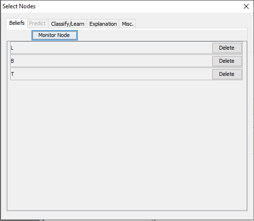
To add a node for recording, click the ‘Monitor Node’ button and the ‘Monitor Node’ dialog appears.

Figure 4: Pick any nodes we wish to record beliefs for and then close the dialog - in this example the nodes from the chest clinic model that represents the diagnosis.

In the ‘Monitor Node’ dialog select a node from the drop down menu. If the selected node is a Discrete Chance Node, select the states you wish to monitor. If the selected node is a Continuous Chance Node, select mean( \(\mu\)) and/or variance ( \(\sigma^2\)). Click the ‘OK’ button to add the node to the list of nodes selected for monitoring.

Figure 5: Pick any nodes we wish to record beliefs for and then close the dialog - in this example the nodes from the chest clinic model that represents the diagnosis.

The nodes selected for monitoring will be listed. Note that if the same node is selected twice it will only appear once in the list as it would otherwise result in duplicate columns in the data set. If a node is selected twice a state which was not previously selected is selected, it will be added to the existing row representing that node.

Figure 6: Pick any nodes we wish to record beliefs for and then close the dialog - in this example the nodes from the chest clinic model that represents the diagnosis.

Depending on the nodes selected, a number of extra columns appear to the data matrix. The information recorded in the column depends on the column name.

Figure 7: Extra columns appear for recording information when a row (a case) is propagated.

In addition to using the above dialog, it is possible to add the columns by hand and specify the appropriate column header to obtain the desired results. There are options to manually specify that the propagate operation should report the probability of a state with maximum probability ([MAX](P(X))) for a discrete chance node, a state with maximum probability ([ARGMAX](P(X))), mean ([MEAN(X)), median ([MEDIAN](X)), quantile ([Qy](X) where 0 < y < 100), probability of an interval [a,b] for a continuous chace node X ([INTERVAL[a,b](P(X))), and coefficient of variance ([CoV](X)) of a numeric discrete node where the format of the column header is shown in parentheses for node X. For instance, to report the mean of X, the column header should be [MEAN](X), to report the coefficient of variance the header should be [CoV](X) and to report the 95 percent quantile the header should be [Q95](X).

To propagate a single row (a case), double click on the row header for the particular row. Alternatively, right click on the row header and select ‘Propagate selected rows’ in the row header menu.

Figure 8: Right-click the row header to enter the row header menu where it is possible to propagate a selected set of rows. Alternatively, to propagate a particular row, double click on the row header for that row.

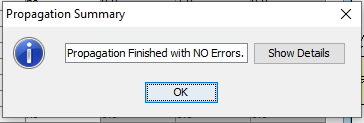
Rows can also be propagated in batch by selecting a number or rows, right-clicking the row header and choose propagate selected rows. Or just right-clicking the row header and choosing propagate ALL rows. When rows are being propagated in batch, a dialog appears displaying the status of the batch propagation job.

Figure 9: Batch propagation job status.

When the batch propagation job completes, information have been recorded for all rows that could be inserted and propagated in the network model.

Figure 10: All rows has been propagated and information recorded.