Data Conflict Analysis

Conflict analysis is the activity of detecting, tracing, and explaining possible conflicts among observations of variable values (i.e., evidence or data). Inconsistencies among observations are easily detected (P(evidence) = 0), but also flawed findings should be detected and traced. For example, in a diagnostic situation a single flawed test result may take the investigation in a completely wrong direction.

Data conflicts are indicated in the right-hand side of the status bar of the Main Window and in the Junction Tree Window (see Figures 1 and 2). Please note that a positive conflict measure indicates negatively correlated observations (i.e., a possible conflict) and that a negative conflict measure indicates positively correlated observations.

Figure 1: The conflict measure computed for the entered evidence is shown in the right-hand side of the status bar of the Main Window.

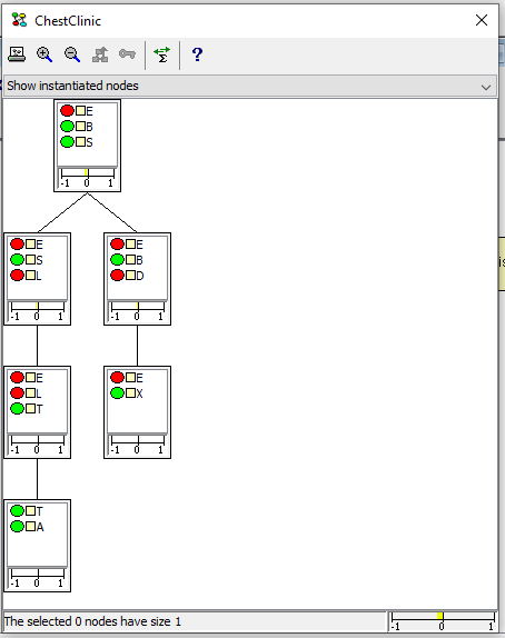
Figure 2: The overall conflict measure computed for the entered evidence is shown in the root clique of the junction tree and in the right-hand side of the status bar of the Junction Tree Window. Local conflicts pertaining to evidence entered in a sub-trees are indicated in the root cliques of these sub-trees.

To understand what conflict analysis is and how it can be used, there are several issues of interest:

• Definition of Data Conflict: How do we define data conflict?

• Conflict Measure: How do we define an appropriate measure of data conflict?

• Conflict Resolution: How do we distinguish between a conflict and a rare case?

• Tracing Conflicts: How do we identify the pieces of evidence that contribute to a data conflict?

Definition of Data Conflict

We define two sets of observations e₁ and e₂ to be in a possible conflict with one another if they are negatively correlated.

For positively correlated findings we expect that P(e_1`|e:sub:`2) > P(e₁) and vice versa (i.e., observing e₂ makes it more likely to also observe e₁ (and vice versa)). In other words, we expect that

\[P(e_1,e_2) > P(e_1)P(e_2)\]

if e₁ and e₂ are positively correlated,

\[P(e_1,e_2) < P(e_1)P(e_2)\]

if e₁ and e₂ are negatively correlated, and

\[P(e_1,e_2) = P(e_1)P(e_2)\]

if e₁ and e₂ are independent.

Conflict Measure

Therefore, given a set of observations (evidence), e = {e₁,…,e_n}, we define the conflict measure for e as

\[conf(e) = log\frac{\prod^{n}_{i = 1} P(e_i)}{P(e)}\]

If conf(e) is positive, e₁,…,e_n are negatively correlated, indicating a possible conflict among these pieces of evidence. (The choice of base for the log function is immaterial.)

Notice, that if conf(e) is negative (i.e., no apparent conflict among e₁,…,e_n), then this gives you no guarantee that all of e₁,…,e_n are positively correlated. It may well happen that there is a local conflict (i.e., that conf(e’) > 0 for a proper subset e’ of e) although conf(e) < 0.

As an example, consider the junction tree in Figure 3, where there are five pieces of evidence (marked by the red nodes). The overall conflict measure is -0.54, indicating no conflict. This measure is obtained from the root clique.

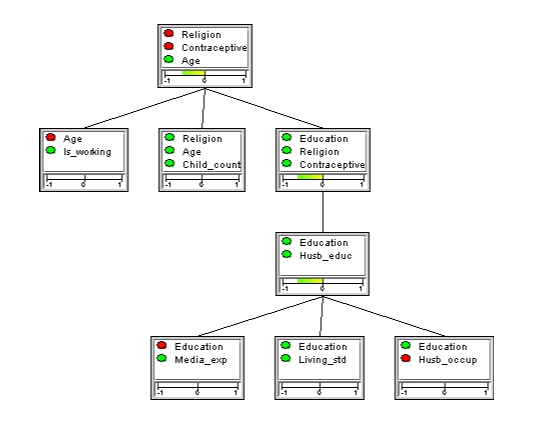
Figure 3: The overall conflict measure for the five pieces of evidence entered (marked by the red nodes) is -0.54, indicating no conflict. Note that the local conflict measure for the two pieces of evidence on Education and Husb_occup (“Husband Occupation”) is less than the overall conflict.

The measure indicated in each clique is the conflict measure pertaining to the evidence entered in the sub-tree with that clique as root. For example, the conflict measure of the clique containing nodes “Education” and “Husb_educ” is -0.6 and pertains to the two pieces of evidence associated with “Education” and “Husb_occup”.

To compute the local conflict measure for the three pieces of evidence associated with “Age”, “Religion” and “Contraceptive” one can select, for example, the clique { “Education”, “Religion”, “Contraceptive” } as root (see Figure 4). (For details on selecting a root of a junction tree, see the Junction Tree section.) Now, it turns out that there is a slight conflict among these three pieces of evidence (conflict measure is 0.39).

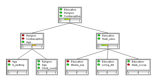
Figure 4: There is a slight conflict among the values observed for the three variables “Age”, “Religion” and “Contraceptive” (conflict measure is 0.39), although there is no overall conflict.

Conflict Resolution

There are situations in which a positive conflict measure is computed, where there is no real conflict. These include:

• Rare case: Typical data from a very rare case may indicate a possible conflict. If conf(e₁,…,e_n) > 0 and there is a hypothesis H=h such that conf(e₁,…,e_n,h) < 0, then h explains away the conflict. That is, if H=h is the correct hypothesis (e.g., a diagnosis) in the current situation, then there is no conflict.

• Missing observation: Basically the same situation, where conf(e₁,…,e_n) > 0 but conf(e₁,…,e_n,I=i) < 0, where I=i is a missing piece of information. That is, there is a local conflict among e₁,…,e_n, but the observation I=i explains the conflict.

By activating the button with the symbol, one can obtain a list of possible instantiations of currently uninstantiated variables that can eliminate the current conflict. The hypotheses are chosen from ones that are set up in the “Hypothesis Variables” tab. An example of the dialog box that appears when this button is activated is shown in Figure 5.

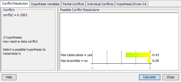
Figure 5: Conflict resolutions dialog box. The box contains a list of possible instantiations of currently uninstantiated variables that can eliminate the current conflict.

The dialog box contains a list of possible instantiations in the form

::

<CM>:<variable>=<value>

where <CM> is the new conflict measure obtained if <variable> is instantiated to <value>. Only instantiations (if any) with a resulting conflict measure less than or equal to 0 get displayed.

The Instantiate button enters the currently selected instantiation (if any) as evidence.

Tracing Conflicts

Whenever a positive conflict has been observed that cannot be explained as a rare case, it is important to pinpoint the piece (or pieces) of evidence that is in conflict with the majority of the pieces of evidence.

Basically, this involves computation of conflict measures for subsets of the evidence. As mentioned and illustrated above, the junction tree is useful for this purpose. As an example, consider the junction tree in Figure 6, where four pieces of evidence have been entered (marked by the red nodes).

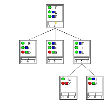
Figure 6: A slight conflict among the pieces of evidence entered (red nodes).

The conflict measure of 0.21 indicates a slight conflict among the these pieces of evidence. To trace the source of the conflict, we can investigate local conflict measures. The junction tree shown above does not reveal any definitive clues as to which piece could be the one causing the conflict. It does show, however, that the local conflict measure is zero for the sub-tree rooted at clique { T, E, L }, indicating that the observations on X and A are not in conflict with one another.

To investigate further, we may select another clique as root of the junction tree, so as to compute some different local conflict measures. If we select clique { T, E, L } as the root of the tree (see Figure 7), we find that there is a slight local conflict among the observed value for D and the observed value for S.

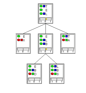
Figure 7: A slight local conflict among the observed values for D and S.