Discretization

Discretization is the task of dividing a set of numerical values into a number of intervals. This task can be performed using the discretization tool. The discretization tool is available for data matrix columns containing numerical data.

When specifying intervals, the lower bound of each interval is inclusive, and the upper bound exclusive - except for the last interval where both lower and upper bounds are inclusive. E.g. If we specify the intervals 0-1, 1-2, 2-3, then the first interval 0-1 would contain all values >=0 and <1, the second interval would contain values >=1 and <2, the last interval would contain values >=2 and <=3.

Intervals must be contiguous, non-overlapping and bound all values in the data to be valid!

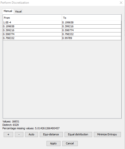
The discretization tool can be seen in Figure 1.

Figure 1: Discretization tool - manualy enter intervals

The top part of the discretization tool has two tabs, Manual and Visual, each providing alternative ways for specifying intervals. From the manual tab, intervals can be entered by hand, and from the visual tab intervals can be defined using a slider.

The bottom part of the tool summarizes a few intersting details about the data, the number of values (not counting missing values), the number of distinct values, and the percentage of missing values.

Below the data summary is a row of buttons for adding and removing intervals, as well as for performing a number of automatic discretization functions.

Function Buttons

Button +

Add interval.

Button -

Remove interval.

Auto

Clicking the Auto button brings forward the auto discretization dialog, see Figure 2. Auto discretization divides the values into a specified number of equally distanced intervals. From the dialog, the number of intervals can be specified, as well as lower and upper bounds and whether to extend bounds to infinity.

Figure 2: Auto discretization dialog - quickly generate a number of equally distanced intervals

Equi-distance

This performs the same kind of discretization as provided by the Auto discretization dialog, just using the current number of intervals.

Equal distribution

This function tries to fit the bounds of the intervals such that each interval contains approximately the same number of values. Depending on how well the data values are scattered, the number of intervals may be pruned in order to make the resulting intervals equally distributed.

Manual

The manual tab contains the table which was seen in figure 1. Each row is an interval, and the columns are the lower and upper bounds for each interval. Intervals are added and removed using the + and - buttons. Upper and lower bounds for an interval is edited by double-clicking the appropriate cell.

Positive and negative infinity are specified using the strings ‘inf’ (for positive infinity), and ‘-inf’ (for negative infinity). Negative infinity is only valid for the lower bound of the first interval, positive infinity is only valid for the closing upper bound of the last interval.

Visual

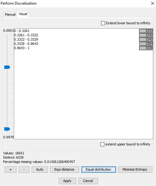
The visual tab contains a list of intervals, and a set of sliders, see Figure 3.

Figure 3: Visual discretization - bars show value count for each interval

The ruler on the left has a slider for each interval. Interval bounds are modified by adjusting the sliders.

The interval list is annotated with bars and value counts. The bars show the proportional number of data values contained in a specific interval. This provided a quick visual overview of how data values are distributed between intervals.

The bars from Figure 3 show an unequal distribution of values between intervals, Figure 4 shows a much better distribution.

Figure 4: Bars show the values are equally distributed between intervals