Auto Filtering (DBN)

With a Dynamic Bayesian network (DBN) loaded HUGIN supports auto filtering from a data file containing a sequence of observations. This is done using the propagation facility in the data frame. To perform Auto Prediction of a DBN start by loading your DBN model. Press Ctrl + O, navigate to the file containing your DBN model and press ‘Open’ and ensure the model is operating in run-mode.

Figure 1: A DBN Model in run-mode. For this example we have loaded machine_monitoring.oobn and configured it with 2 time slices (using the Network Properties Panel).

By following these links you can read how to:

• open your data file,

• associate you data file with a run-mode DBN model,

• point out the Sequence Identifier if you have multiple sequences in you data file, and

• convert the data to time windows.

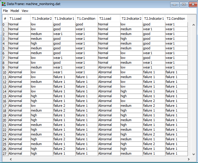
When you have completed these steps your data frame should look something like the content in Figure 2. Here the data file is assumed to contain a single sequence and thus a Sequence Id is not specified.

Figure 2: The content of the data frame when the file machine_monitoring.oobn was loaded and converted to a sequence of time windows.

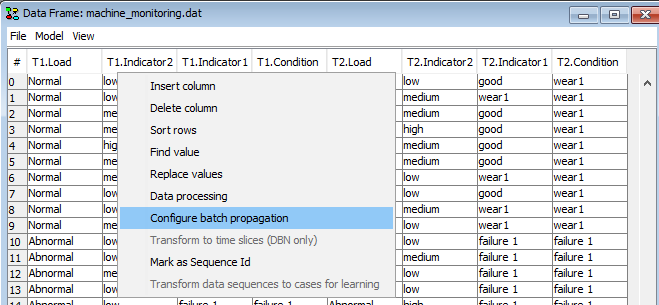
To perform filtering right click on a column header and select ‘Configure batch propagation’ (Figure 3) to access HUGIN’s Batch propagation configuration menu in the data frame.

Figure 3: Select Configure batch propagation to enter the batch propagation configuration dialog.

Navigate to the ‘Predict’ tab, click ‘Add Belief’ and configure a new prediction on the Time slice and Variable you wish to perform filtering on. For this example, assume you have the model in Figure 1 and you wish to perform Bayesian filtering on T1.Condition and T2.Condition (states ‘failure 1’ and ‘failure 2’). Then add 2 predictions with Node=Condition, and states ‘failure 1’ and ‘failure 2’ for time slice 1 and 2 respectively. Eventually, you should obtain the screen in Figure 5.

Figure 4: Configure batch propagation by adding 2 predictions on nodes T1.Condition and T2.Condition.

Figure 5: The Batch propagation configuration dialog with the filters added.

To propagate the data, right-click on a row header and select “Propagate ALL rows” or “Propagate selected rows”. To read more about propagation of data in DBN models, click here! Answer ‘Yes’ when you are asked whether the variables should be ignored in the filtering (Figure 7).

Figure 6: Propagate the data by right-clicking on a row header and selecting “Propagate ALL rows”.

Figure 7: Answer ‘Yes’ when you are asked whether the variables should be ignored in the filtering.

You can use HUGIN’s Classifier Performance tool to get an indication of how well the model has performed. Right-click in a cell and select ‘Classifier Performance’.

Figure 8: To evaluate how well the variable was predicted, right-click in a cell and select ‘Classifier Performance’

• As ‘Actual Class’ select one of the columns you renamed previously to leave them out of the batch propagation.

• As ‘Target Class’ select one of the states in the ‘Actual Class’ column that you just selected.

• As ‘P(Target Class’) select the column which contains the propagated belief of the ‘Target Class’ you just selected.

Figure 9: ROC curve indicating the performance of the Bayesian filter on the node T1.Condition.