Auto Prediction (DBN)

With a Dynamic Bayesian network (DBN) loaded HUGIN has the ability to perform auto prediction from a data file containing a sequence of observations. This is done using the propagation facility in the data frame. To perform Auto Prediction of a DBN start by loading your DBN model. Press Ctrl + O, navigate to the file containing your DBN model and press ‘Open’ and ensure the model is operating in run-mode.

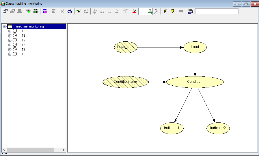
Figure 1: A DBN Model in run-mode.

Now open your data file containing your data sequence. To open a new data frame and load a data file, click in the menu of the main HUGIN frame File -> Open Data File and select a data file. The file is assumed to be in csv format.

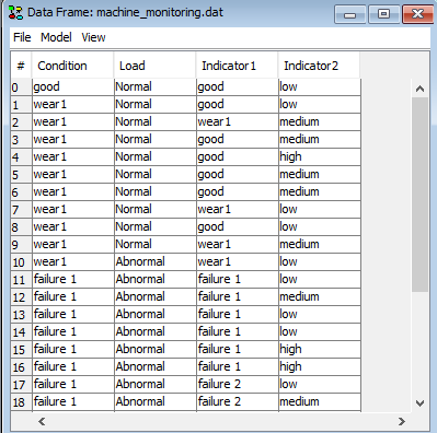
Figure 2: The Data sequence loaded in HUGIN’s Data Frame.

Note the auto prediction functionallity is only available in the dataframe if it has been associated with a DBN model in run-mode!

To associate the data frame with your DBN Model in run-mode, click the Model menu and then click Select a Run-Mode Model. A dialog appears, containing all the current project frames to pick from.

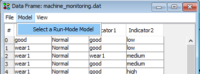
Figure 3: To associate the data sequence with the DBN model select ‘Select Run-Mode Model’ form the ‘Model’ menu.

Figure 4: Pick a project for doing the DBN auto Prediction.

Convert your data file to a sequence of time windows if the data you have loaded is not already in the auto prediction time window format. To do this, right click a column header in the data matrix and select Transform to time slices (DBN only).

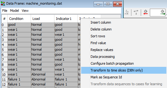
Figure 5: Select configure batch propagation (Note: if this option is dimmed out, then switch the associated network model to run-mode first).

The dialog in Figure 6 will appear asking you how you wish to align your data and whether you wish to keep or replace the original columns in the dataset.

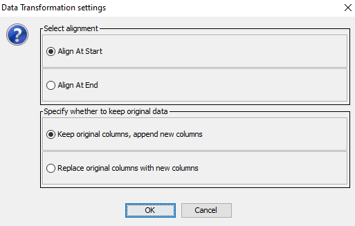
Figure 6: A dialog will appear asking how to align the original data in the time slices and whether the original columns should be replaced.

When the tool performs a transformation it consults the associated run-mode model when it looks for the following parameters:

• Time Slices: The number of time slices in the run-mode DBN model determines the time horizon of the transformed data set.

• Node Names: The column headers in the original time series data must be equal to the corresponding the node names in the run-mode DBN model. Columns without a corresponding node name will be ignored.

Let T be the number of Time Slices configured in the associated run-mode DBN and N be the number of columns for which the column header equals a node name in the associated run-mode DBN and finally, let the columns in the original time series data with matching nodes in the associated model be labeled n₁, n₂, … n_N. Then the process generates T * N columns as following: “T1.n₁”, “T1.n₂”,…”T1.n_N”, “T2.n₁”,…, “TT_N”.

The data in each case is transformed from a time series to a sequence of horizon time windows with horizon T.

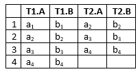
Thus, if we for instance have a datafile with a time series over the variables A and B as follows:

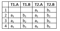
If the associated run-mode model is a DBN with 2 time slices over the variables A and B, the conversion produces:

• If “Align at Start” has been choosen:

• If “Align at End” has been choosen:

The result of the transformation in the machine_monitoring.dat and machine_monitoring.oobn files which can be found in the example folder is outlined in Figure 7.

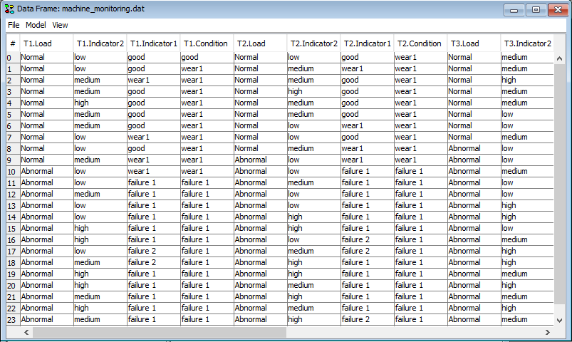
Figure 7: Outline of the result from transforming machine_monitoring.dat with machine_monitoring.oobn loaded as DBN run-mode model.

To configure which variable to target for prediction right-click on a column header in the data frame window and select ‘Configure batch propagation’.

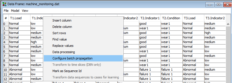
Figure 8: Select ‘Configure batch propagation’ in the table header menu in order to specify which variables to predict.

In the Select Nodes dialog navigate to the ‘Predict’ tab and click ‘Add Prediction’ to specify a new variable for prediction.

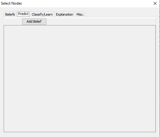
Figure 9: Click ‘Add Prediction’ to specify a new variable for prediction.

In the ‘Add Prediction’ dialog, specify which variable and which timeslot you wish to predict.

Discrete valued chance nodes, Continuous chance nodes, Discrete Function Nodes, and Continuous Function Nodes can be selected for prediction.

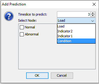
Figure 10: Select time slice, node and states which should be marked for prediction.

When a variable has been selected, further parameters can be selected for the prediction. If the node is a discrete chance node or a discrete function node the desired states can be marked for prediction. To mark all states select the variable twice in the ‘Select Node’ drop down menu.

Note: As soon as you click ‘OK’ your choices will be stored in the dataframe. A new column will be added for each selected state. (See ‘How Predictions are stored in the dataframe’ to understand how this works).

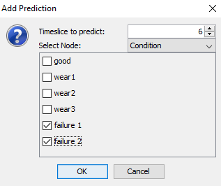
Figure 11: Press ‘OK’ to store your selection and corresponding columns will be added to the data frame.

You can add as many Prediction elements as you want. If you add a new prediction element with the same variable and time slice as an existing prediction element the selected states will be ‘absorbed’ by the existing element and a new element will not be added to the list but new columns will be added for each new selected state (See ‘Predictions are stored in the dataframe’).

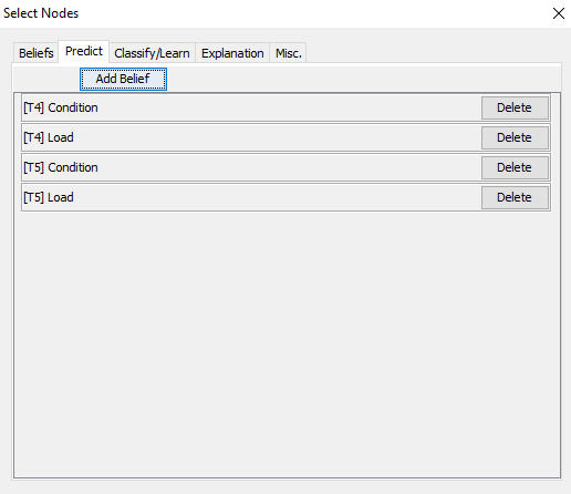
Figure 12: You may add as many prediction elements as you like. The predictions you select are immediately added as new columns in the data frame.

Predictions are stored as columns in the dataframe. Assume that each individual state s1 , s2 , … sn for node N in timeslot t are marked for predicition using the ‘Add Prediction’ dialog. Then a columns with a headers [T_t]P(N=s₂), [T_t]P(N=s₂),…[T_t]P(N=s_n) are added to the data in the data frame.

An example excerpt of the the machine_monitoring.dat and machine_monitoring.oobn examples from the HUGIN Example folder with states selected for prediction is outlined in Figure 13.

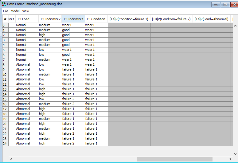
Figure 13: An example excerpt of the the machine_monitoring.dat and machine_monitoring.oobn examples from the HUGIN Example folder with states selected for prediction.

To perform the propagation of the selected timeslots, variables and states right click on a row-header and you now have two possibilities:

• Select either ‘Propagate selected rows’ to propagate either the selected row or a subset of rows in sequence. Prior to this choice, the rows you wish to propagate must be selected with the mouse: Hold down left mouse button over the first or last row you wish to select and pull either up or down,

• or select ‘Propagate ALL rows’ to propagate all cases stored in the data frame in sequence.

Note

The order in which the rows are propagated matters. Each time a row is propagated, the time window offset is advanced with 1 time step in the associated run-mode DBN model and all evidence will be accumulated. This corresponds with entering the evidence in the model window and pressing (move time window) which will affect the result of all subsequent propagations. If you start a propagation of any number of rows and the time window offset is not 0 you will see the warning in Figure 16 but the system will proceed with the prediction. This allow interleaved batch propagation of subsets of cases in the data frame and manual interaction with the model for inspecting the propability distributions in the model at a particular state.

If this is not desired, it is highly recommended to press (compile) which will reset the time window offset to 0 and then use the ‘Propagate ALL rows’ option.

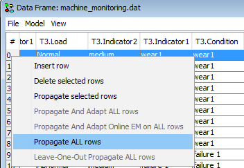
Figure 14: The recommended way to perform propagation is to press (compile) in the run-mode DBN model which will reset the time window offset to 0 and then use the ‘Propagate ALL rows’ option.

During the batch propagation you will see the progress. To stop the propagation simply close the progress window.

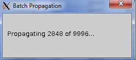
Figure 15: The progress window shown during the batch propagation. To stop the propagation simply close the progress window.

Figure 16: If you start to propagate a number of rows and the time window offset is not in state 0 you will see this warning but the propagation will proceed as soon as you press ‘Yes, Continue!’.

The propagated values will be written to the respective cells in the data matrix.

Figure 17: The propagated probabilities will be written to the cells in the data frame. Cells will be overwritten when the rows are propagated again.

To Evaluate a prediction HUGIN’s Data Processing Tool and HUGIN’s Data Classifier Performance Tool can be used. First the rows containing the true future values must be aligned with the prediction in the data set. This can be obtained using HUGIN’s Data Processing Tool .

To align the rows containing the true future values with the predictions open the Data Processing Tool by right clicking on a column header in the data frame and select Data Processing (Fig. 18).

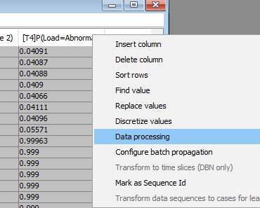
Figure 18: To open the Data Processing Tool right click on a column header and select Data Processing.

When The Data Processing Tool appears press ‘+’ to create a new Data Processor. You can edit the Data Processor directly in the Details section in the dialog window below.

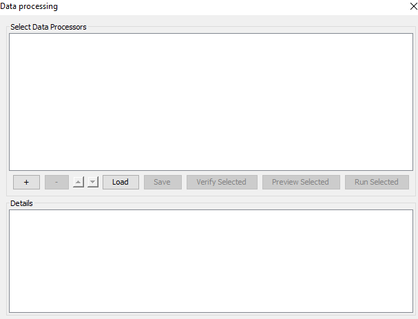
Figure 19: The Empty Data Processing Tool. Press ‘+’ to create a new Data Processor. You can edit the Data Processor directly in the Details section in the dialog window below.

Assume you have a runtime model and a dataset with 3 time slices (i.e. T1, T2 and T3) and you have added a prediction on a variable in the future time slice T4. To align the true future data with the predictions in T4 you wish to copy the data in the T1 columns and shift them 4 cells up. The following 2 Data Processor Descriptions can obtain this when run in sequence:

To clone all columns in time slice T1 (T1.A, T1.B,…) and name them with prefix “eval-T4-” (eval-T4-T1.A, eval-T4-T1.B, …) use the following data processor description:

COLUMN_CLONE
SELECT T1.*
eval-T4-

To obtain this, press ‘+’, select ‘<Empty Data Processor Template>’ and enter the above text in the Details section. To shift all columns with prefix “eval-T4-” 4 cells up use the following data processor description:

COLUMN_SHIFT
SELECT eval-T4-.*
4
UP

To obtain this, press ‘+’, select ‘<Empty Data Processor Template>’ and enter the above text in the Details section. When you have entered both data processing descriptions you should see something like Figure 20 where the 2 new data processors are listed.

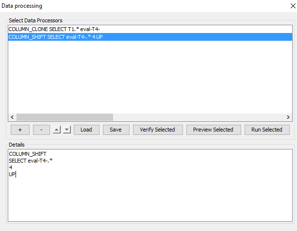
Figure 20: The Data Processing Tool with the 2 above processors entered.

To run the data processors select the two processors by holding down the CTRL key while selecting them in the list and press ‘Run Selected’. If it ran successfully you should obtain the dialog in Figure 21. You can now close the Data Processing Tool and verify that the columns should have been added and shifted as requested (See Figure 22).

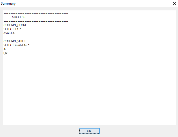
Figure 21: You should see this information .

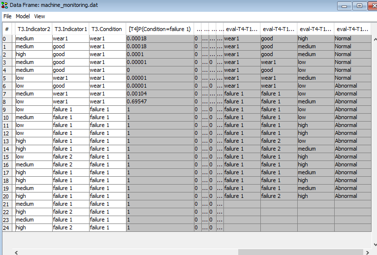
Figure 22: The columns have been cloned and shifted such that the predicted values are aligned with the actual future values.

The predictions can be evaluated using the HUGIN’s Data Classifier Performance Tool. To open this tool right click one of the cells in the Data Frame and select ‘Classifier Performance’ as shown in Figure 23. This shoul open the Classifier Performance Tool shown in Figure 24.

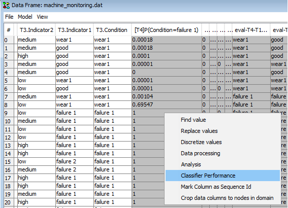
Figure 23: Right click on a data cell and select ‘Classifier Performance’ to evaluate the prediction.

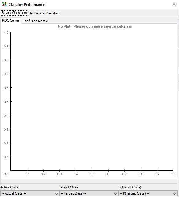
Figure 24: The Classifier Performance Tool. The tool is configured by selecting the three evaluation parameters in the bottom of the window.

Configure the classification by selecting values for the three parameters at the bottom of the Classifier Performance window:

• Actual Class: Select the column containing the actual future value. Assume we wish to evaluate the performance of the prediction labelled “[T4]P(Condition=failure1)” and that we have used the data processors described above. Then the column labelled “eval-T4-T1.Condition” contains the actual values that “[T4]P(Condition=failure1)” predicts.

• Target Class: Select the state that the prediction we are evaluating predicts. If we are evaluating “[T4]P(Condition=failure1)” then select “failure1”.

• P(Target Class): Select the column containing the prediction. In this case select “[T4]P(Condition=failure1)”.

The result of this configuratin is shown in Figure 25. The ROC curve appears as soon as the last value is selected.

If you need to see more details about the prediction, navigate to the “Confusion Matrix” tab to see a count of false positives and false negatives and other relevant parameters (See Figure 26).

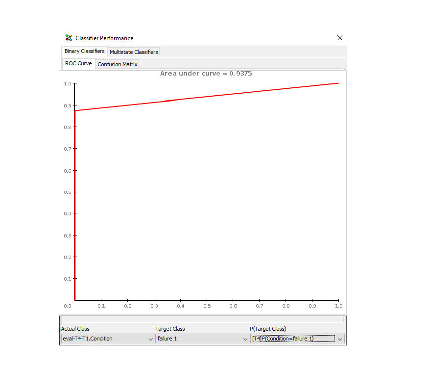
Figure 25: The resulting ROC Curve indicating the performance of the prediction.

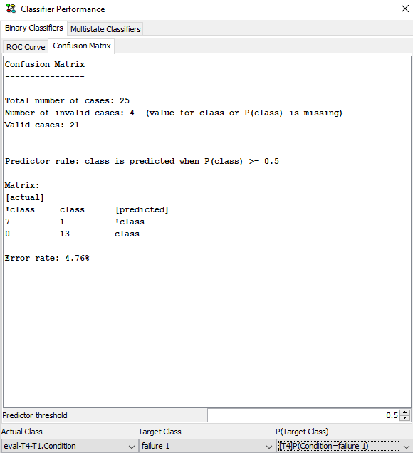
Figure 26: The confusion matrix for the prediction.