The Exposure, Occurrence and Impact Loss Model

The XOI Loss Model dialog allows the user to compute a loss distribution based on the eXposure, Occurrence, and Impact Loss Model (XOI Loss Model). A XOI loss distribution can be computed by either MC simulation or by convolution of impact and exposure/frequency distribution.

What is the XOI Loss Model?

The XOI Loss Model computes a total impact distribution based on exposure, occurrence, and impact.

• Exposure is a quantitative specification of the number of independent objects at risk.

• Occurrence is a Boolean specification of the occurrence of an event on one exposed object during one period.

• Impact is a quantiative specification of the severity of the occurrence of an event on one specific object.

The occurrence node is a Boolean chance node, the impact node is an interval node, and the exposure node is a numbered or interval node. Based on the states and distributions of exposure, occurrence, impact a total impact distribution is calculated. This distribution assesses the risk related to all exposed objects. The distribution is computed with respect to an interval node referred to as total impact. This node is created by HUGIN.

Figure 1 shows the XOI Loss Model dialog.

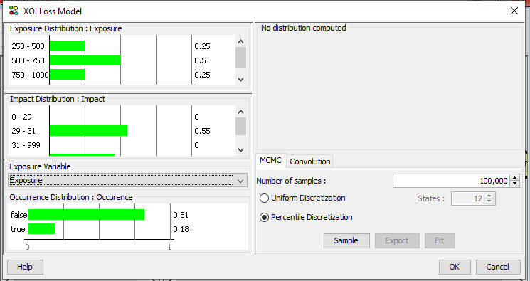
Figure 1: The XOI Loss Model dialog.

The calculation of the loss distribution under the XOI Loss Model is a two step process. In the first step a (large) number of samples or tiny intervals with associated probability are generated. In the second step the samples or tiny intervals are used as the basis for identifying the intervals of total impact.

There are two models for generating the samples (we refer to the tiny intervals generated as samples too) of total impact: the MCMC model and the Convolution model. Under the MCMC model the samples are simulations of the values of total impact while under the Convolution model the samples are (tiny) intervals of total impact with an associated probability (i.e., samples are not sampled values, but correspond to a very fine-grained discretization of total impact. As mentioned, we refer to these intervals as samples). In each case a large number of samples should be generated when a high accuracy is desired.

There are some requirements that must be fulfilled under the XOI Loss model:

• The first state of impact must include zero.

• The numbered and interval nodes must be well-formed. The interval node is well-formed when its intervals cover a positive range including zero (and it otherwise meets the requirements for an interval node).

• The exposure node can either be numbered or interval, but it must be positive, i.e., its states must specify positive values.

A few details on the implementation applying to both the MCMC and the Convolution algorithm:

• Once a value of exposure is determined, the posterior beliefs of impact and occurrence are updated, i.e., a full evidence propagation is performed. This implies that the distribution of each other node is conditioned on the value of exposure.

• If an interval has a probability mass larger than 10%, then it is not possible to perform the percentile fitting operation.

• It is important for the user to make sure that the probability associated with semi-infinite intervals are small (in order to minimize their influence on the calculations).

• When two interval nodes and one Boolean node are selected the user may have to change the choice of exposure (and impact) node.

• We do not allow evidence exposure, impact, and occurrence.

The MCMC Model

Under the MCMC model the loss distribution, i.e., the posterior probability distribution of total impact, is calculated based on Monte-Carlo simulation. A large number of samples are generated conditional on exposure and other evidence. The distribution of total impact is calculated as the accumulated loss.

Each sample is generated as follows. First a value of exposure is sampled. Then we sample the remaining variables n times where n is the sampled value of exposure (holding the value of exposure fixed). If occurrence is true, we accumulate the value of impact. The exposure node is sampled as many times as specified by the user. Each sampled value of total impact requires as many samples as specified by exposure. The final accumulated value is the desired sampled result.

The Convolution Model

Under the Convolution model the loss distribution, i.e., the posterior probability distribution of total impact, is calculated based on the convolution of a frequency and an impact distribution.

The convolution function computes the convolution of a frequency distribution and an impact distribution. We use the convolution function to compute the distribution of total impact where a Binomial distribution is used as the frequency distribution. That is, the frequency distribution is simulated using a Binomial distribution with parameters n and p. The parameter n is equal to a value of exposure and the parameter p is equal to the probability of Occurrence being true. The convolution algorithm is based on the Table Generator implementation, i.e., when exposure is an interval node we for each interval use a predefined number of values in the calculations (as opposed to only using the middle value of an interval).

The initial number of bins is set to 10000 and the maximum loss is set to maximum exposure times maximum loss. The initial value of maximum loss may be too large when the probability of occurrence is low. When the maximum loss is too large a large number of intervals will be assigned zero probability. In this case the maximum loss can be reduced in order to obtain a more fine-grained initial discretization of total impact. Figure 2 shows the XOI Loss Model dialog once the Convolution tab is selected by the user.

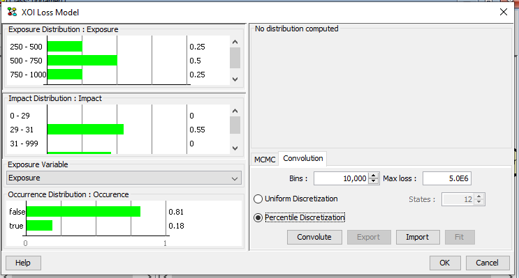
Figure 2: The XOI Model dialog once the Convolution tab is selected by the user.

Once the user selects to convolute the tool generates the samples for total impact. Figure 3 shows samples generated for total impact.

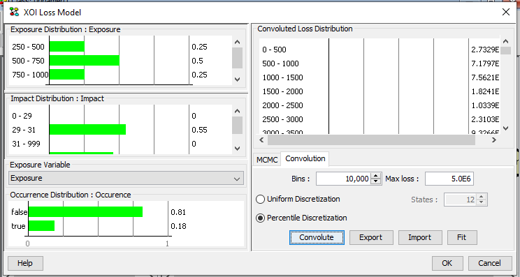
Figure 3: The samples generated once the user selects to convolute.

The samples generated for total impact can be fitted to a (significantly) reduced number of intervals. This fitting operation is a discretization process. The user has to select how the discretization should be performed. The user can either choose to perform a uniform discretization (and specify the number of states) or a percentile-based discretization (an example of the percentile-based discretization is show in Figure 4).

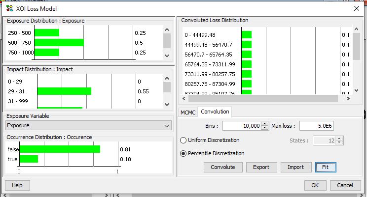
Figure 4: The distribution of total impact as a result of convolution.

Figure 4 shows the distribution of total impact as a result of convolution.