Analysis Wizard

The Analysis Wizard performs several kinds of analysis on a network; Based on a set of cases the wizard will calulate the AIC-, BIC- and log-likelyhood scores, perform various data dependency and accuracy analysis.

The Analysis Wizard is activated by selecting “Analysis Wizard” in the Wizards Menu. Note that to activate the Analysis Wizard, the network must be in runmode and consist only of discrete chance nodes.

When the Analysis Wizard is activated a window displaying the “Data Source” pane will pop up, see figure 1. The window has six tabs: “Data Source, “AIC/BIC/ll”, “Dependencies”, “Data Accuracy”, “Sampling” and “Cases/Beliefs”.

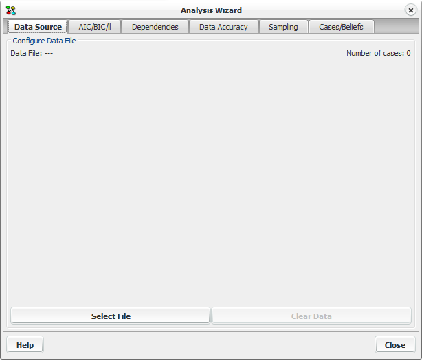
Figure 1: Empty Data Source pane; Window displayed when the Analysis Wizard is activated.

Data Source pane

To perform any analysis the wizard will first need a set of cases. Cases can be imported by

• loading a HUGIN data file,

• or sampling a number of random cases.

Click on button “select file” to load a HUGIN data file or click on the tab “Sampling” to sample a number of random cases to use as data source.

Sampling pane

Clicking on the tab “Sampling” will bring forward the sampling pane. The sampling pane is shown in figure 2.

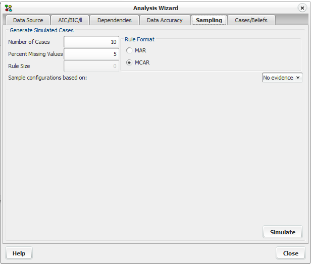
Figure 2: Sampling pane.

Cases can be generated in two different ways: MCAR (Missing Completely at Random) or MAR (Missing at Random). MCAR sets some values to N/A by removing values of some nodes in the generated case set randomly (i.e., MCAR considers all the values in the generated cases and not one case at a time).

MAR randomly sets some values in a case to N/A based on auto-generated templates. These templates specify that if some nodes have a specific value, then the values of a subset of the nodes are randomly set to N/A. Note that the specification of the templates is generated randomly.

In both cases the conditional probability distribution is considered as a factor to the number of cases generated with a specific set of observations. Also in both MCAR and MAR it is possible to indicate the percentage of missing values.

The cases generated will be based on the conditional probability distribution given by the scenario chosen in the combo box “Sample configurations based on”.

Any cases generated will be added to the current set of imported cases.

AIC/BIC/ll pane

Clicking on the “AIC/BIC/ll” tab will bring forward the AIC/BIC/ll pane, see figure 3. The wizard calculates the AIC, BIC and log-likelihood scores of the model given the case data.

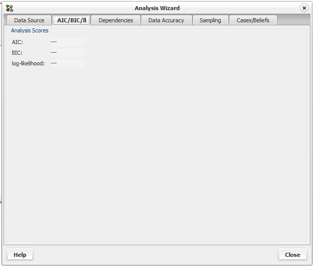
Figure 3: AIC/BIC/ll pane.

Dependencies pane

Clicking on the “Dependencies” tab will bring forward the data dependencies pane, see figure 4.

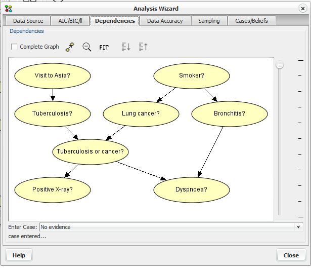
Figure 4: Data dependencies pane.

The Dependencies pane allow for inspecting the mutual information of nodes. Depending on the threshold set by the slider, edges will be hidden according to the mutual information of the nodes. Toggle between inspecting mutual information for all nodes or nodes with directed edges by clicking the checkbox “Complete graph”. Mutual information will be computed based on the case selected in the “Enter Case” drop down box.

Buttons at the top of the pane allows for zooming the view of the network and adjusting the scale of the slider if possible.

• Stronger and weaker dependencies can be identified by moving the threshold slider, as edges are only displayed if the mutual information between the connected nodes are above the threshold.

• Mutual information between all nodes can be inspected by clicking ‘Complete Graph’.

• Mutual information computation will be based on the the network instantiation chosen in the ‘Enter Case’ drop-down list

Data Accuracy pane

Clicking on the “Data Accuracy” tab will bring forward the Data accuracy analysis pane, see Figure 5. Given a node and a set of cases, this pane generates an analysis report with information about how well the predictions of the network match the cases.

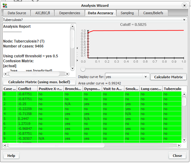
Figure 5: Data Accuracy pane.

This pane consists of four elements, a drop down box at the top to select what node to analyze, an ROC curve, an analysis report and a table showing the cases.

Analysis Report

The analysis report list the number of cases used for analysis (only cases without observations of the actual node is ignored). A confusion matrix is generated showing how well the observed states match the predicted. For prediction we can use either of the following options:

1. random state with the highest belief to be the predicted state*.

2. specific state with a belief greater than or equal to the ROC cutoff threshold.

• (if a node has two or more states that qualify to be the predicted state, one of them is randomly selected as the predicted state)

The button Calculate Matrix (using max. belief) makes a report where prediction is based on (1). Selecting a specific state and threshold for the ROC curve and clicking the button Calculate Matrix makes a report where prediction is based on (2).

The report also contains a number of distance measures, the average euclidian distance and Kulbach-Leibler divergence. The distance measures are from the true distribution x inferred from the case data e with respect to the selected node X, and the distribution y resulting from propagating eX.

The Euclidian distance is computed as:

\[dist_Q(x, y) = \sum_{i}(x_i - y_i)^2\]

The Kulbach-Leibler divergence is computed as:

\[dist_K(x,y) = \sum_{i}(log_2 x_i - log_2 y_i)^2\]

The reported distance measure is averaged over all cases where X has been observed.

ROC Curve

The ROC curve lets you inspect the performance of a given variable as a classifier for the data set. X-axis is the false positive rate, and the Y-axis is the true positive rate. The ROC curve is based on the performance for predicting specific states. The area under the can be used as a measure for the “goodness” of the network as a classifier for the given variable. The button Calculate Matrix generates a report based on the selected curve and ROC cutoff threshold as described above in Analysis Report. The threshold can be specified by moving the threshold slider left and right. The current threshold is also signified by a point on the curve, signifying the expected performance with regards to the ratio between true and false predictions.

Case table

The table shows the cases used for analysis. The node selected for analysis will always be located in the second last column of the table. The last column in the table report the probability of the node being in the state observed in the case, given the case without information about the state of the node itself. Cases are colored green for a match, red for no match and blue if ignored and orange if unable to make a prediction. A match is when the predicted state for the node is the same state observed in the case.

Case Beliefs pane

Clicking on the “Cases/Beliefs” tab will bring forward the cases pane, see Figure 6. The case pane offers the option of selecting a node and one of it’s states and displaying the beliefs for that state in each case, highlighted by a color.

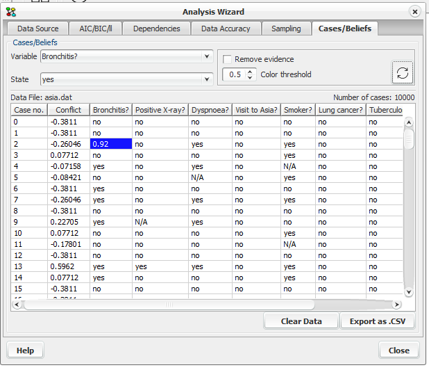
Figure 6: Cases - Beliefs pane

This pane consists of six elements, a drop down box at the top to select what node to analyse, a dropdown box to select one of the node’s states, a check box (Remove evidence), the color threshold spinner, a refresh button and a table showing the cases.

By selecting a node and one of its states, the case table displays the beliefs for that node in each case for which no evidence is entered. The information for the selected node will always be displayed in the first column after the “Case no.” column (second column).

By checking the Remove evidence check box and pressing the refresh button, beliefs are retracted and displayed for cases where evidence was entered in the node under analysis

The color threshold spinner offers the option of selecting the belief values to be colored (the values higher than the selected are colored). The tone of the color indicates how high the value is (the darker the color the higher the value is). The coloring ability together with the ability to sort the column makes it easier to notice the values desired.

To sort the column click, once on it’s header for ascending order or twice for descending. It is possible to save one or more cases to a file so they can be used in another wizard (f.ex Parameter Sensitivity). After selecting one or more cases right click on the mouse and select “Save Case” for saving one case, or “Save Selected Cases” for saving many cases. (see Figure 7).

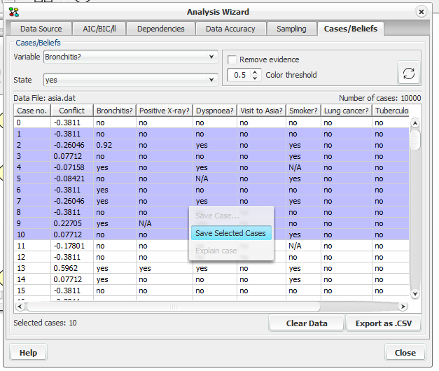
Figure 7: Cases - Beliefs pane “save selected cases”