Monitor Windows

In Run Mode you can open Monitor Windows for all or some of the nodes. You can choose the Toggle Monitors item from the Network Pane Menu which is activated when you press the right mouse button somewhere in the network pane while working in Run Mode. You can also select the nodes and press the monitor icon on the top left of the network pane. There are three types of monitor windows (see Figure 1, Figure 2, and Figure 3) - one for each of the node types: discrete chance node, continuous chance node, and decision node. You cannot open a monitor window for a utility node.

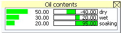
Figure 1: A monitor window for a discrete chance node.

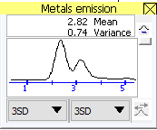
Figure 2: A monitor window for a continuous chance node.

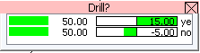
Figure 3: A monitor window for a decision node.

A monitor window shows the computed results (i.e., posterior marginal distribution and expected utility function) for a node:

• Discrete chance nodes: The probability of each state. In a LIMID both the probability and the expected utility of each state under the current strategy are shown.

• Continuous chance nodes: The mean, variance (SD), and the PDF (probability density function) graph.

• Decision nodes: The probability and expected utility of each action (decision option) under the current strategy.

Monitor windows for continuous chance nodes can open with or without showing the graph display below the pane showing mean and variance (depending on the settings in Network Properties as described below). You can open and close it by clicking the small button on the right of the mean and variance. You can chose different end points as the mean plus/minus an integral multiple of the variance from the two drop down lists below the pane containing the graph.

On the right side of the graph there is a slider which can be used to zoom in on the x-axis to spot local peaks on the graph. Just below this slider is a button which should be pressed after each propagation to update the graph if auto update of graphs is not enabled. HUGIN does not automatically update the graphs because this could take a very long time for large networks.

You can customize the monitor windows to your needs in the Monitors tab of the Network Properties dialog box. Figure 4 shows the Monitors tab.

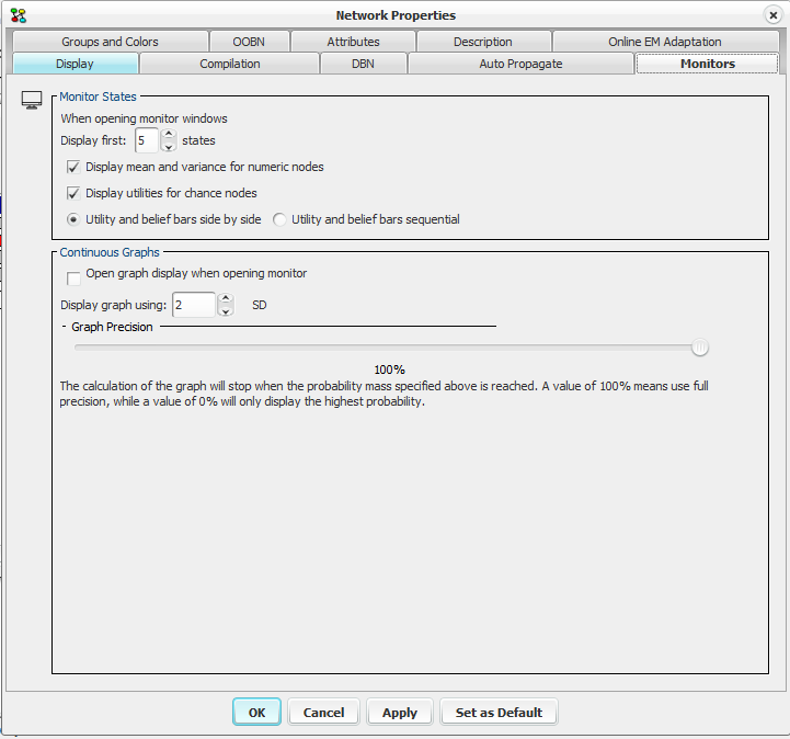
Figure 4: The Network Properties dialog box showing the Monitors tab.

You can configure the monitors to show at most a certain number of states in the Monitor States group box. For continuous chance nodes, you can specify if you always want the monitor to open with the graph pane and you can specify the end points (in multiples of the variance) of the graph.

It is also possible to configure monitors to display means and variance for numeric nodes (See Figure 5), whether utilities should be displayed for chance nodes (LIMIDs) and whether Utilities and Belief bars should be arranged side by side or in sequence.

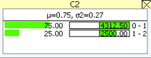
Figure 5: A Numeric node shown with Mean and Variance.

You can also specify the graph precision. Normally, you would want the graph as precise as possible but if you have a large network with many continuous chance nodes and poor performance, you might save some time if you decrease graph precision. Different display modes are available for the monitor windows. For discrete chance nodes there are four different modes:

Normal Mode. This is the default mode, showing the current marginal distribution for the node. Relative Difference Mode. This mode shows the relative change of each probability with respect to what it was before new evidence was inserted and propagated. The change is displayed in percent. Absolute Difference Mode. This mode shows the absolute change of each probability with respect to what it was before new evidence was inserted and propagated. Mixed Mode. This mode is similar to Normal Mode, except that below each bar is shown another (slimmer) bar indicating the probability before new evidence was inserted and propagated. Display mode is changed by right-clicking on the monitor, and by selecting “Display Mode” (Figure 6).

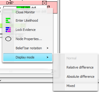
Figure 6: The Normal Mode before evidence has been entered and propagated.

Figure 7 shows a monitor in Normal Mode for a discrete chance node before evidence is entered and propagated.

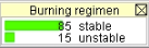
Figure 6: The Normal Mode before evidence has been entered and propagated.

Figure 8 shows the same monitor in Normal Mode after evidence has been entered and propagated.

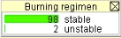
Figure 7: The Normal Mode after new evidence.

Figure 9 shows the monitor in Relative Difference Mode after the evidence has been entered and propagated.

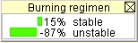
Figure 9: The Relative Difference Mode after new evidence.

Figure 10 shows the monitor in Absolute Difference Mode after the evidence has been entered and propagated.

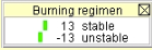
Figure 10: The Absolute Difference Mode after new evidence.

Figure 11 shows the monitor in Mixed Mode after the evidence has been entered and propagated.

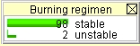
Figure 11: The Mixed Mode after new evidence.

For continuous chance nodes there are two different modes:

1. Normal Mode. This is the default mode, showing the current marginal density function for the node.

2. Mixed Mode. In this mode, both the new an the old marginal density functions are shown.

Please note that selection of display mode for continuous monitors has effect only when the monitor is expanded, showing the marginal density function (i.e., the display mode has no effect on the mean and variance values shown in the upper part of the monitor).

Figure 12 shows a monitor in Normal Mode for a continuous chance node before evidence is entered and propagated.

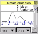
Figure 12: The Normal Mode before evidence has been entered and propagated.

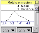
Figure 13: The Normal Mode after new evidence.

Figure 14: The Mixed Mode after new evidence.

For decision nodes there are two different modes:

1. Normal Mode. This is the default mode, showing the probability and expected utility for the each decision option for the node.

2. Absolute Difference Mode. This mode shows the absolute change in the probability and the expected utility for each decision option with respect to what it was before new evidence was inserted and propagated.

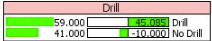
Figure 15: The Normal Mode before evidence has been entered and propagated.

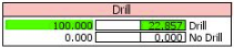
Figure 15: The Normal Mode after new evidence.

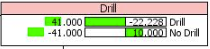
Figure 16: The Absolute Difference Mode after new evidence.

Display modes are selected through the popup menu that appears when right-clicking a monitor window.